- Suggested problems for Section 7.4: 3, 7, 11, 13, 14, 15, 17, 21
- Suggested problems for Section 7.3: 1, 3, 5, 9, 11, 12
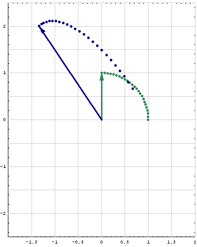
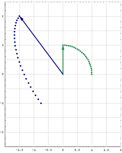
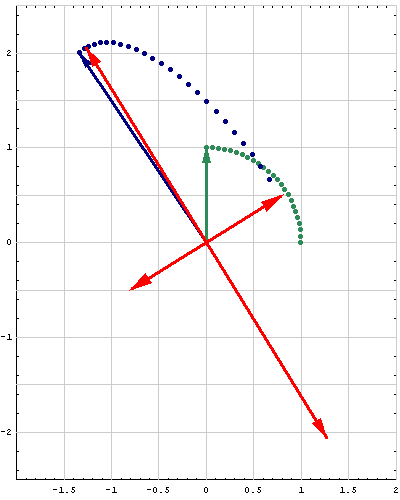
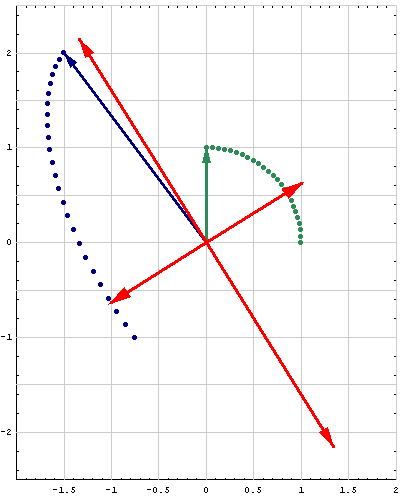
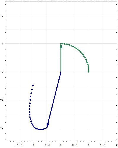
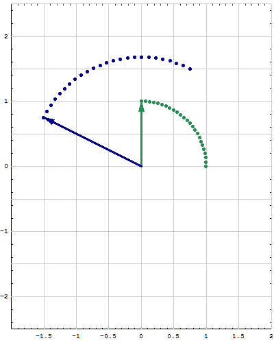
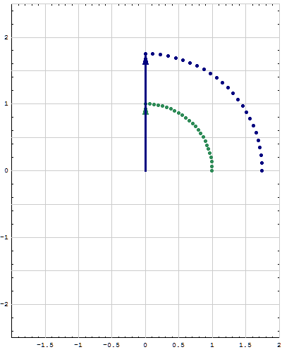
- With what we learned in 7.3 we can go back to the animations from the beginning of the quarter and calculate some remarkable quantities that appear naturally in those animations. Here is one animation that is at the beginning of the bottom of this page and a new one. Looking at the blue vectors bellow we see that their heads trace an ellipse. What are the directions and lengths of their axes? Based on what we learned in 7.3 we can calculate these quantities.
- In the animations below we emphasize the direction and the lengths of the axes of the ellipses traced above. You should understand how these quantities are calculated.
-
Going back to Section 7.2, in the book they do not discus quadratic forms with three variables. This is usually done in Math 224. Here are some animations that might help you understand the quadratic form $x_1^2 + x_2^2 - x_3^2$. Here I show the surfaces in ${\mathbb R}^3$ with equations $x_1^2 + x_2^2 - x_3^2 = c$ for different values of $c$.
Place the cursor over the image to start the animation.
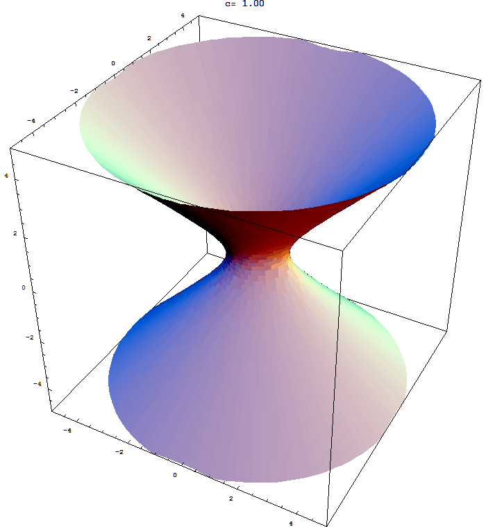
Five of the above level surfaces.
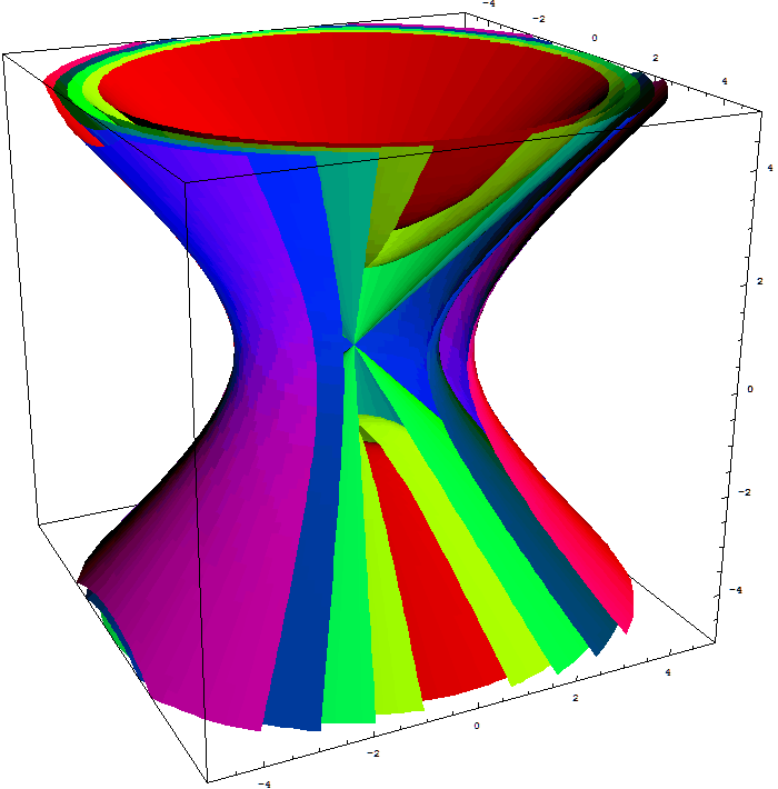
Place the cursor over the image to start the animation.
|
|
|
|
- This is the Mathematica notebook that I used today. It contains a $3\times 3$ illustration of the Spectral Theorem for symmetric matrices. I also added three $4\times 4$ illustrations.
- Suggested problems for Section 7.2: 1, 3, 5, 7, 9, 13, 17, 19, 20, 21, 23, 25
- Suggested problems for Section 7.1: 3, 4, 9, 11, 15, 19, 23, 24, 25, 27, 30, 31, 32, 33, 35, 36, 37
- Suggested problems for Section 6.8: 1, 2, 5, 6, 7, 9, 10, 11, 14
- This is the Mathematica notebook that I used today.
- Suggested problems for Section 7.1: 3, 4, 9, 11, 15, 19, 23, 24, 25, 27, 30, 31, 32, 33, 35, 36, 37
- Suggested problems for Section 7.2: 1, 3, 5, 7, 9, 13, 17, 19, 21, 23, 25
- Suggested problems for Section 7.3: 1, 3, 5, 9, 11, 12
- Suggested problems for Section 7.4: 3, 7, 11, 13, 14, 15, 17, 21
- Suggested problems for Section 6.8: 1, 2, 5, 6, 7, 9, 10, 11, 14
- This is the Mathematica notebook that I used today.
- Suggested problems for Section 6.7: 1, 2, 3, 5, 7, 9, 10, 13, 16, 17, 19, 20, 21, 23, 25
- Suggested problems for Section 6.6: 1, 2, 3, 4, 5, 6, 7, 8, 9, 14, 15, 16
- This is the problem I stated today in class: Let $m$ and $n$ be positive integers. Let $A$ be an arbitrary $m\times n$ matrix. There are 12 vector spaces related to the matrix $A$ that are of interest. Those are \begin{alignat*}{3} & {\rm Col}\, A & & {\rm Row}\, A & & {\rm Nul}\, A \\ & ({\rm Col}\,A)^\perp\, \qquad & & ({\rm Row}\, A)^\perp \qquad & & ({\rm Nul}\,A)^\perp \\ & {\rm Col}(A^T) & & {\rm Row}(A^T) & & {\rm Nul}(A^T) \\ & \bigl({\rm Col}(A^T)\bigr)^\perp\, \qquad & & \bigl({\rm Row} (A^T)\bigr)^\perp \qquad & & \bigl({\rm Nul}(A^T)\bigr)^\perp \\ \end{alignat*} First identify each of the 12 subspaces as a subspace of ${\mathbb R}^n$ or ${\mathbb R}^m$. Then identify the subspaces that are equal. What is the largest number of genuinely distinct subspaces that can occur in the above list? What is the smallest number of genuinely distinct subspaces that can occur in the above list?
- Suggested problems for Section 6.5: 1, 3, 6, 7, 9, 13, 16, 17, 19, 20, 21, 22
- Suggested problems for Section 6.4: 2, 3, 5, 7, 9, 13, 15, 17, 19, 20
- Here is the Mathematica notebook that I used today. It is just the calculations, but you should be able to understand the content in which calculations are done.
- Suggested problems for Section 6.3: 1, 2, 4, 5, 7, 10, 11, 13, 15, 16 17, 19, 20, 21, 23
- Suggested problems for Section 6.4: 2, 3, 5, 7, 9, 13, 15, 17, 19, 20
- Suggested problems for Section 6.2: 2, 3, 5, 8, 9, 11, 13, 15, 17, 19, 21, 23, 25, 26, 27, 29.
- To understand the importance of dot product you need to review Law of cosines. Here is Wikipedia's Law of cosines page. Wikipedia offers six different proofs. Find one that resonates best with you. Have you seen this proof in high school? Which one?
- Here is an additional problem for Section 5.6. Given the matrix $A$ and the vector ${\mathbf{x}}_0$ given by \[ A = \begin{bmatrix} 2 & -3/2 \\ 1 & -1/2 \end{bmatrix}, \quad {\mathbf{x}}_0 = \begin{bmatrix} 3 \\ 4 \end{bmatrix} \] and consider the difference equation ${\mathbf{x}}_{k} = A {\mathbf x}_{k-1}, \ k\in{\mathbb N}$. Find the solution of this difference equation. That is, find an explicit formula for ${\mathbf x}_{k}$ depending only on $k$. Determine the limiting value for ${\mathbf x}_{k}$ as $k\to +\infty$.
- Suggested problems for Section 6.1: 1, 5, 7, 8, 9-12, 13, 15-18, 20, 22, 24, 25, 26, 27, 28, 29, 31
- Suggested problems for Section 5.6:1, 2, 3, 4, 5, 6, 9, 12, 13, 15
- Here is the Mathematica notebook that I used today.
- Suggested problems for Section 5.5: 1-6 (Are these matrices in "The book of Beautiful Matrices"?), 7-12, 13, 16, 17, 18, 21, 25, 26
- The Book of Beautiful Matrices consists of two-by-two matrices whose entries and eigenvalues are integers between -9 and 9. I consider only the matrices with the nonnegative top-left entry. In addition, I consider only matrices with the relatively prime entries. To get matrices that are omitted in this way you just multiply one of the given matrices by an integer. You need to adjust the eigenvalues by multiplying them with the same integer. The eigenvectors remain unchanged.
- I divided the Book in three volumes: Volume 1 contains matrices with real distinct eigenvalues, Volume 2 contains matrices with non-real eigenvalues (whose real and imaginary part are integers between -9 and 9) and Volume 3 contains matrices with a repeated eigenvalue. The eigenvalues and a corresponding eigenvector (and a root vector for repeated eigenvalues) are given for each matrix. Three volumes in pdf format are here:
- Suggested problems for Section 5.4: 1, 3 - 13, 17, 19 - 23, 27, 28
- As we see everyday in class the identity matrix is very important. Let $n \in {\mathbb N}$. The identity matrix of size $n$ is the $n\times n$ square matrix with ones on the main diagonal and all the other entries are zero. It is denoted by $I_n$, or simply by $I$ if the size is clear from the context in which matrix appears. \[ I_1 = \begin{bmatrix} 1 \end{bmatrix} ,\ I_2 = \begin{bmatrix} 1 & 0 \\ 0 & 1 \end{bmatrix} ,\ I_3 = \begin{bmatrix} 1 & 0 & 0 \\ 0 & 1 & 0 \\ 0 & 0 & 1 \end{bmatrix} ,\ \cdots ,\ I_n = \begin{bmatrix} 1 & 0 & \cdots & 0 \\ 0 & 1 & \cdots & 0 \\ \vdots & \vdots & \ddots & \vdots \\ 0 & 0 & \cdots & 1 \end{bmatrix} \] In the problem below we consider the reverse identity matrix, or anti-identity matrix. The reverse identity matrix, denoted by $J_n$, is the matrix in which the columns of the identity matrix $I_n$ are written in reversed order: the last column of the identity matrix is the first column of the reverse identity matrix: \[ J_1 = \begin{bmatrix} 1 \end{bmatrix} ,\ J_2 = \begin{bmatrix} 0 & 1 \\ 1 & 0 \end{bmatrix} ,\ J_3 = \begin{bmatrix} 0 & 0 & 1 \\ 0 & 1 & 0 \\ 1 & 0 & 0 \end{bmatrix} ,\ \cdots ,\ J_n = \begin{bmatrix} 0 & \cdots & 0 & 1 \\ 0 & \cdots & 1 & 0 \\ \cdot & \ \ \ \ \cdot & \cdot & \cdot \\ \cdot & \cdot & \cdot & \cdot \\ \cdot & \cdot \ \ \ \ & \cdot & \cdot \\ 1 & \cdots & 0 & 0 \end{bmatrix} \] Sometimes the anti-identity matrix $J_n$ is described as the n�n square matrix with ones on the diagonal going from the lower left corner to the upper right corner and all the other entries are zero. It is a very special case of an anti-diagonal_matrix.
-
This is the assignment problem:
Let $n \in {\mathbb N}$ be arbitrary. Prove that the reverse identity matrix $J_n$ is diagonalizable. In solving this problem a concept of a block matrix might be useful.
The solution is due in class on July 5, 2011. Since I did quite a bit of this problem in class, your solution must be complete, well justified, consistent with the definitions and well written to receive the full credit.
- Suggested problems for Section 5.3: 1, 3, 5, 6, 7, 8, 15, 17, 18, 21, 22, 23, 26, 27, 28, 31
-
Today in class I demonstrated how to use Mathematica to calculate eigenvalues and eigenvectors. Here is the Mathematica file that can help you repeat those calculations. The file is called Matrix.nb. Right-click on the underlined word "Here"; in the pop-up menu that appears, your browser will offer you to save the file in your directory. Make sure that you save it with the exactly same name. After saving the file you can open it with Mathematica. You need to find a campus computer with Mathematica installed on it (for example BH 209, BH 215). You will find Mathematica as follows (this sequence might differ on different campus computers)
Start -> Programs -> Math Applications -> Mathematica. Open Mathematica first, then open Matrix.nb from Mathematica. You can execute the entire file by the following manu sequence (in Mathematica):Kernel -> Evaluation -> Evaluate Notebook. There are some more instructions in the file. - More information on how to use Mathematica you can find on my Mathematica page.
- If you have problems running files that I posted please let me know. If you spend some time learning how to use Mathematica you will enhance your understanding of math that we are studying.
- Suggested problems for Section 5.2: 1-8 (find corresponding eigenvectors as well), 9, 13, 15, 18, 19, 20, 21, 24, 25, 27
- A related Wikipedia link: Characteristic polynomial. Wikipedia's presentation is slightly different from ours.
- A new room has been assigned for the class. It is CB 485, Chemistry Building. Tomorrow we will meet in this room.
- The information sheet
- Suggested problems for Section 5.1: 1, 3, 4, 5, 6, 8, 11, 15, 16, 17, 19, 20, 24-27, 29, 30, 31
- A related Wikipedia link: Eigenvalue, eigenvector and eigenspace.
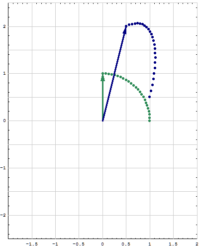
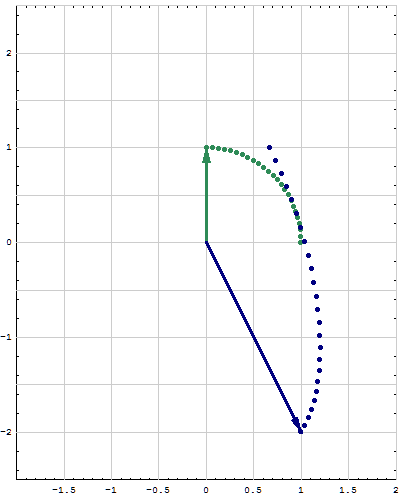
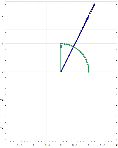
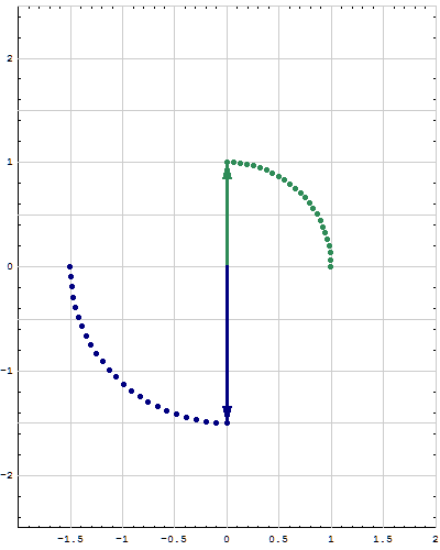
- Here are animations of different matrices in action. In each scene the navy blue vector is the image of sea green vector under multiplication by a matrix A. For easier visualization of the action the heads of the vectors leave traces. Just looking at the movies you can guess what the matrix is in each movie. You can also see what its eigenvalues and eigenvectors are, whether an eigenvalue is positive, negative, zero, complex, ...
Place the cursor over the image to start the animation.
|
|
|
|

|
|
|
|