Assignment 1
Problems by Branko Curgus
In[121]:=
![]()
Prolog to Problem 1. Two cylinders
This is a tribute to a problem that I was assigned as an undergraduate student in the mid-1970s at the Department of Mathematics of the University of Sarajevo.
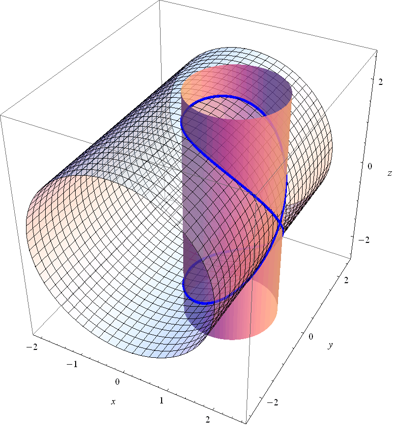
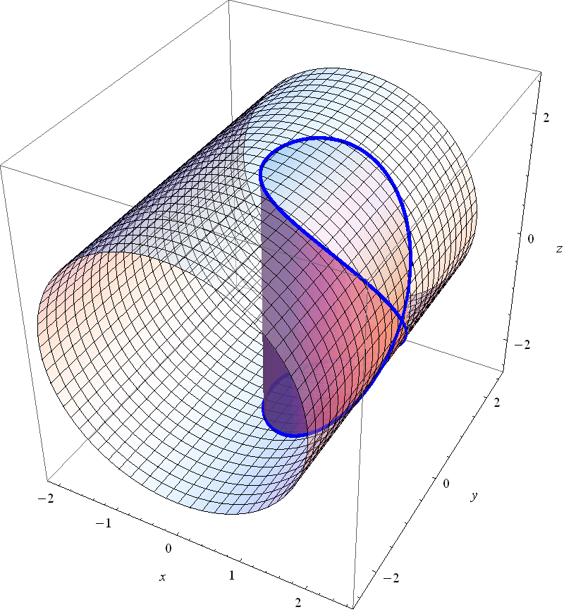
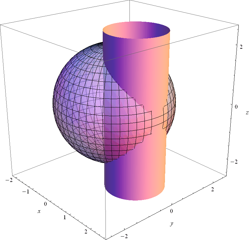
The problem involves the intersection of two circular cylinders. The smaller cylinder is vertical with the equation: ![]() (this is the circle centered at (1,0) with the radius 1) and z is arbitrary. The larger cylinder is horizontal with the equation:
(this is the circle centered at (1,0) with the radius 1) and z is arbitrary. The larger cylinder is horizontal with the equation: ![]() and y is arbitrary. I do not recall exactly what I was asked to do with these two cylinders. However, I remember well that I spent a lot of time trying to visualize the intersection. At that time I did not have access to any technology to help with visualization.
and y is arbitrary. I do not recall exactly what I was asked to do with these two cylinders. However, I remember well that I spent a lot of time trying to visualize the intersection. At that time I did not have access to any technology to help with visualization.
Since I do not recall what was the exact question related to these two cylinders I will calculate all quantities that come to mind related to this object.
Visualization
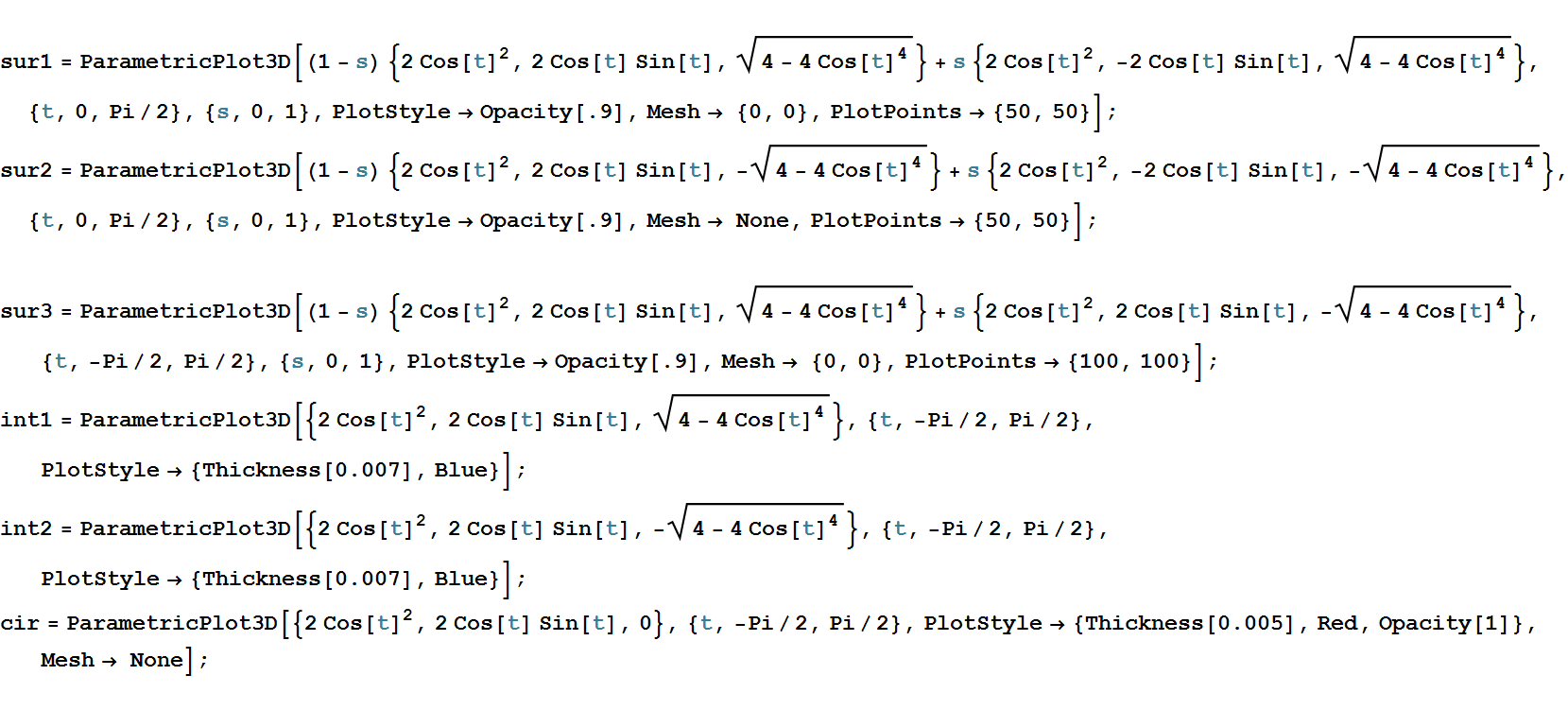
This is a convenient view point in the graph below which I determined through experimentation.
In[1]:=
![]()
Out[1]=
![]()
In[2]:=
Out[8]=
In[9]:=
In[14]:=

Out[14]=
In[15]:=

Out[15]=
In[16]:=
Out[20]=
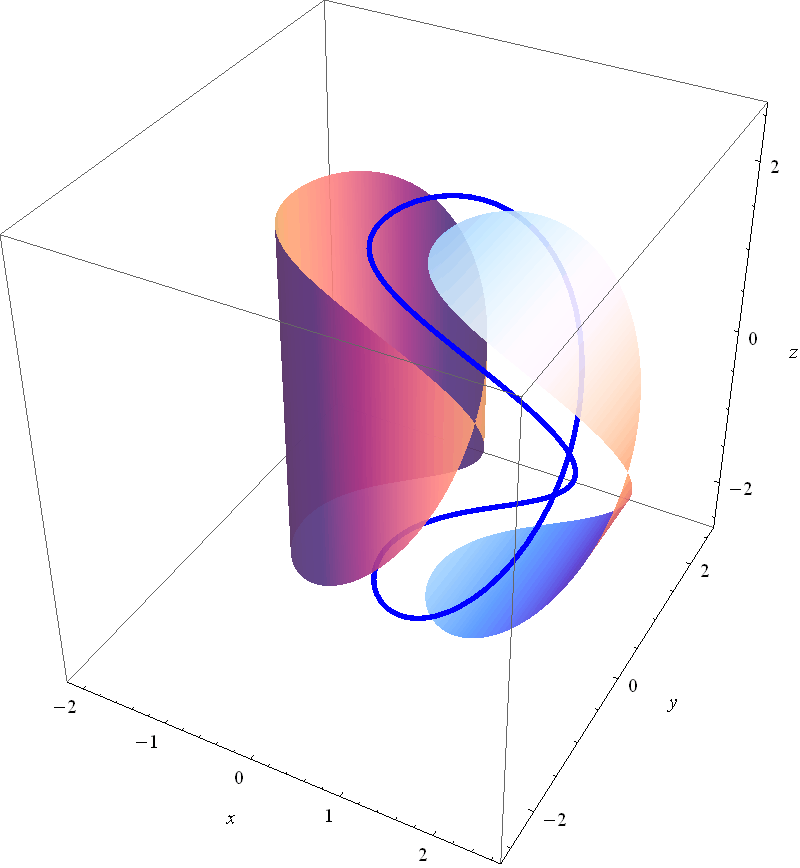
Unwrapping
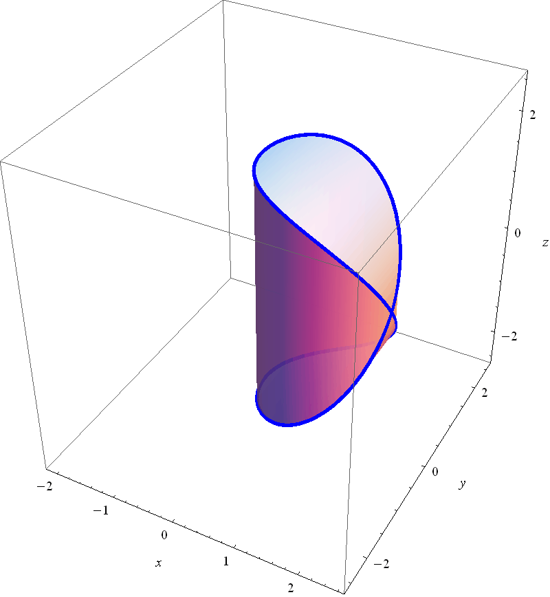
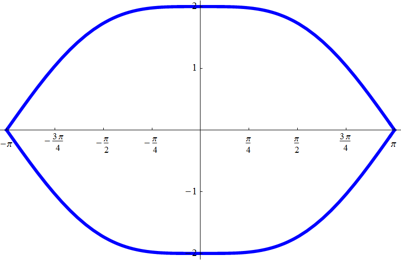
Each cylinder can be unwrapped to a plane. Hence the blue curve above and two surfaces bounded by the blue curve can be unwrapped into planes.
How to find the equation for the blue curve when unwrapped to a plane? The following picture can help.
In[21]:=

Out[21]=
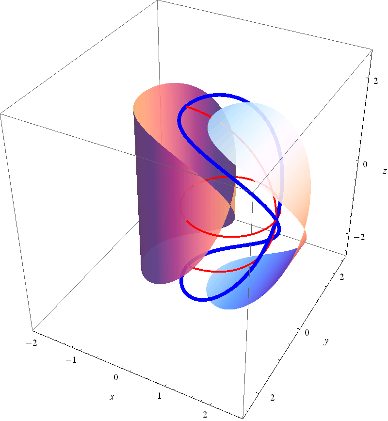
Large cylinder
Let us consider first unwrapping the blue curve into the plane by unwrapping the larger cylinder. As the larger cylinder is unwrapped to a plane, the vertical red half-circle is unwrapped to a vertical line segment of length 2π. The parametric equation of the top part of the blue curve is
![]()
The equation of the red horizontal circle is
![]()
and the blue curve is above the red horizontal circle and on the large cylinder whose top part is given by ![]() .
.
Now we will determine the equation of the top part of the blue curve in relation to the arc length on the vertical red circle. Let P be the point on the vertical red circle such that s is the arc length between the point (2,0,0). The coordinates of P are (2 Cos[s/2], 0, 2 Sin[s/2]). Which point on the blue curve has the same z-coordinate? Call that point B. The point B has the same x-coordinate as P. Thus,
![]()
Solving for t we get
In[22]:=
![]()
![]()
Out[22]=

Substituting

in
![]()
In[23]:=

Out[23]=

This expression can be further simplified to
In[24]:=

Out[24]=

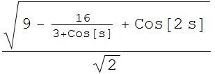
Thus, the blue point B is at the distance  from the point P. Thus, when flattened the equation of the blue curve is as follows:
In[25]:=

Out[25]=
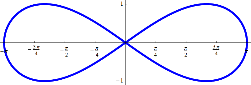
It is interesting to point out that the equivalent expression for the blue curve above is as follows
In[26]:=

Out[26]=
![]()
Small cylinder
Now we will unwrap the blue curve by unwrapping the smaller cylinder. As a parameter we will take the arc length s along the horizontal red circle starting from (2,0,0). As before, call P the point on this circle such that the arc length between P and (2,0,0) is s. From the geometry of the unit circle it follows the polar angle θ for this point is θ = s/2. Therefore this point is given as
![]()
The parametric equation for the top part of the blue curve is
![]()
Thus the point on the blue curve vertically above the point P is

In[27]:=

Out[27]=
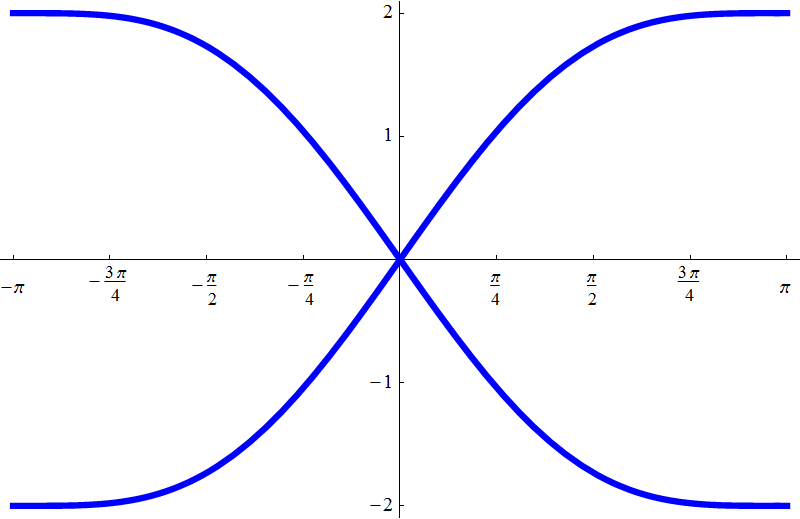
Or, cutting the surface at the point (2,0,0).
In[28]:=

Out[28]=
Calculations
The surface area of the eight-shaped region
This is the surface area on the larger cylinder. It is the transparent surface in the picture. The area is
In[29]:=

Out[29]=
![]()
In[30]:=
![]()
Out[30]=
![]()
A different way to calculate this surface is to use the surface integral.
In[31]:=

Out[31]=

In[32]:=

Out[32]=

In[33]:=
![]()
Out[33]=
![]()
In[34]:=

Out[34]=

In[35]:=

Out[35]=
![]()
In[36]:=
![]()
Out[36]=
![]()
Exactly the same value.
The vertical surface area
We found the equation so we just integrate.
In[37]:=

Out[37]=
![]()
In[38]:=
![]()
Out[38]=
![]()
This expression can be simplified by hand to
In[39]:=
![]()
Out[39]=
![]()
In[40]:=
![]()
Out[40]=
![]()
It is interesting to point out that the above formula for the blue curve has equivalent form as follows:
In[41]:=

Out[41]=
![]()
In[42]:=

Out[42]=

In[43]:=

Out[43]=
![]()
A different way to calculate this surface is to use the surface integral. I was not able to get the exact value in this way, just an approximation.
To get equation for the surface
In[44]:=
![]()
Out[44]=
![]()
In[45]:=

Out[45]=

In[46]:=

Out[46]=

We need to integrate this quantity over the half circle in xz-plane
In[47]:=

But this integral is not evaluating.
Try for the indefinite integral, that is anti-derivative:
In[48]:=

Out[48]=
![]()
Now use the Fundamental Theorem of Calculus
In[49]:=

Out[49]=

And integrate numerically:
In[50]:=

Out[50]=
![]()
The volume
To calculate the volume we integrate the big cylinder over the small disk:
In[51]:=

Out[51]=

In[52]:=

Out[52]=
![]()
Or the small cylinder over the big half-circle. I was not able to get the exact value in this way.
In[53]:=
![]()
In[54]:=

Out[54]=

In[55]:=

Out[55]=
![]()
The length of the blue curve:
We first use the first parametrization in the plane obtained above:
In[56]:=

Out[56]=

In[57]:=

Out[57]=
![]()
The second parametrization in the plane
In[58]:=

Out[58]=
In[59]:=

Out[59]=
![]()
Finally we use the parametrization of the blue curve in space:
In[60]:=

Out[60]=
![]()
In[61]:=

Out[61]=

In[62]:=

Out[62]=

In[63]:=

Out[63]=
![]()
One more parametrization in space
In[64]:=

Out[64]=

In[65]:=

Out[65]=

In[66]:=

Out[66]=
![]()
Problem 1: Your task
Repeat as much as you can of what I did in Prolog to Problem 1 when the large Cylinder is replaced by the sphere of radius 2 centered at the origin
In[67]:=
![]()
Out[67]=
![]()
In[68]:=

Out[70]=
Prolog to Problem 2. Two famous multiple integrals
A famous double integral
Consider the integral  .
.
Mathematica does calculate this integral.
In[71]:=

Out[71]=
![]()
However, calculating this integral by hand using the Fundamental theorem of calculus is not easy. Here is why
In[72]:=

Out[72]=

This is doable by hand. Now we apply the FTC and get
In[73]:=

Out[73]=

Next we integrate
In[74]:=

Out[74]=
![]()
But this integral is a special function that is not familiar to an undergraduate student. In fact this is not often studied function.
Applying FTC again we get.
In[75]:=

Out[75]=
![]()
Our goal is to understand this result using change of variables in double integral.
We use the following change of variables:
![]()
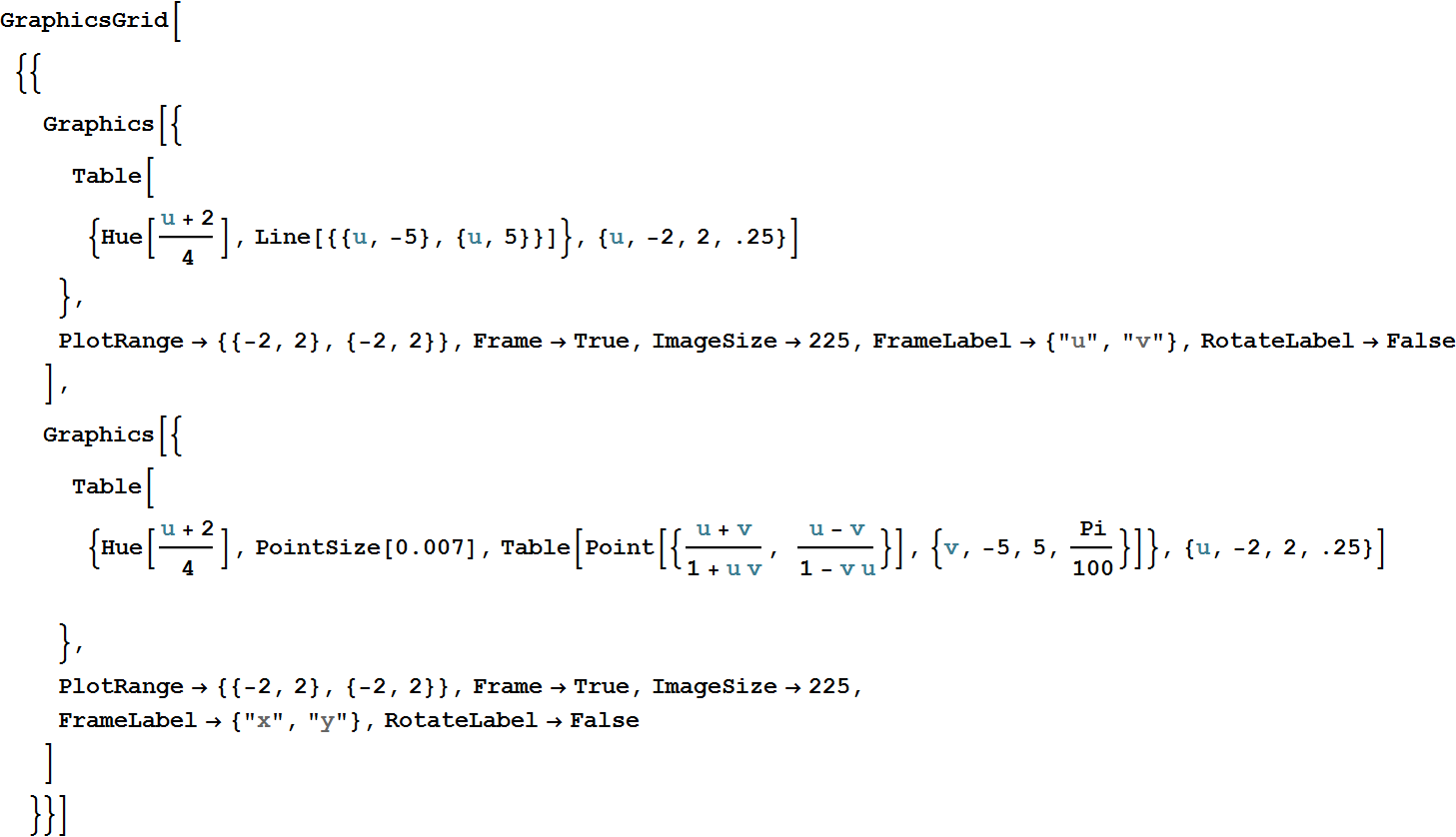
Good way to think about this change of variables is as a mapping from uv-plane into xy-plane.
![]()
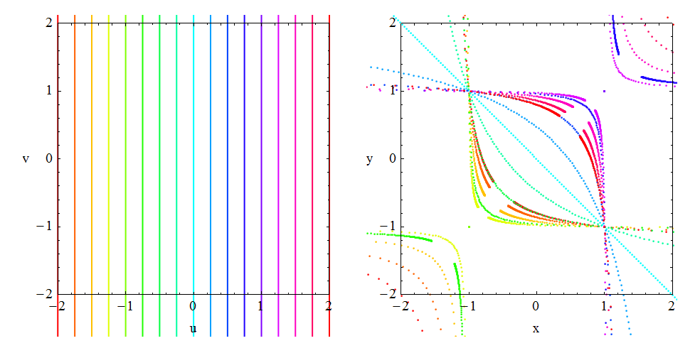
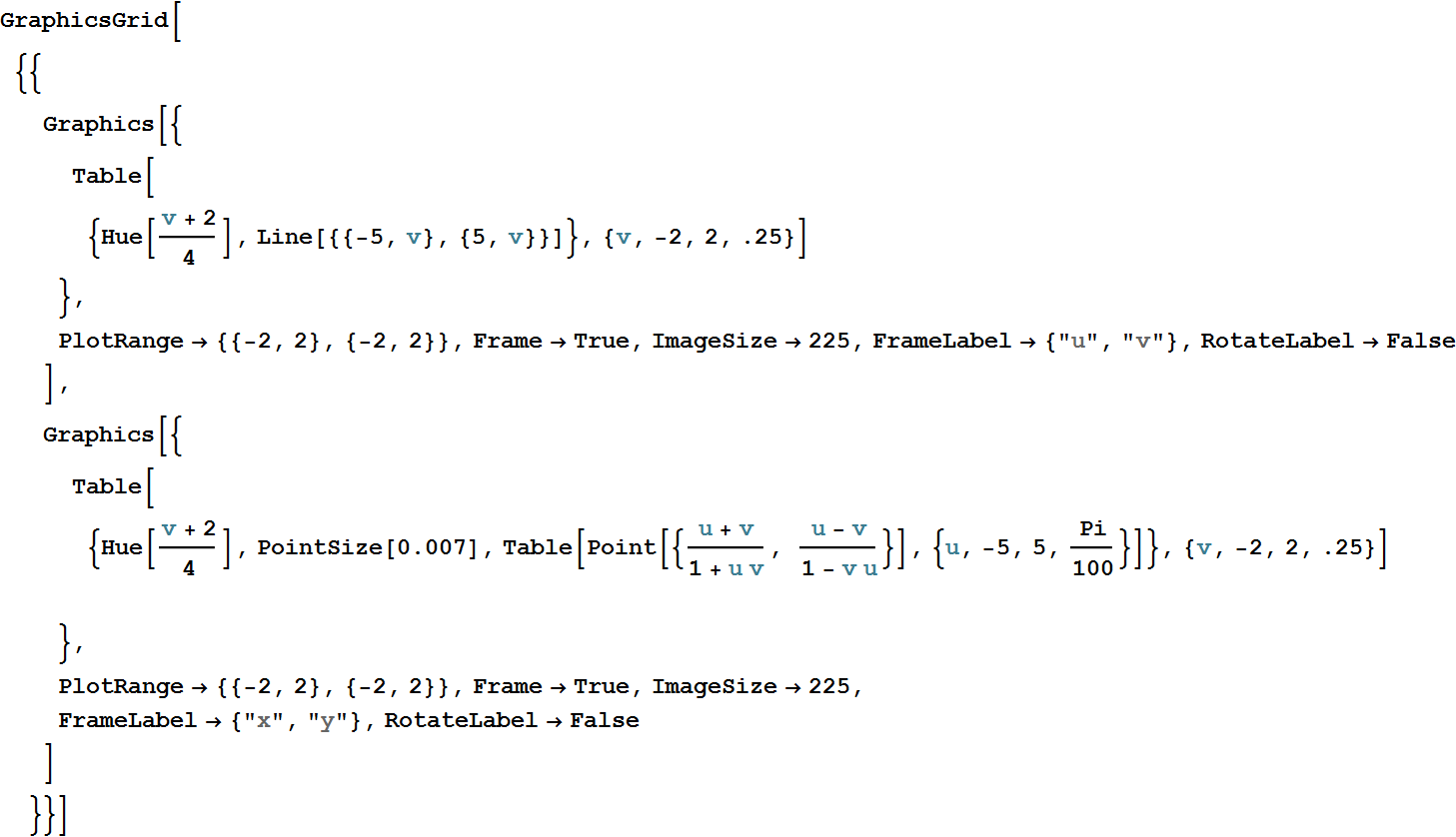
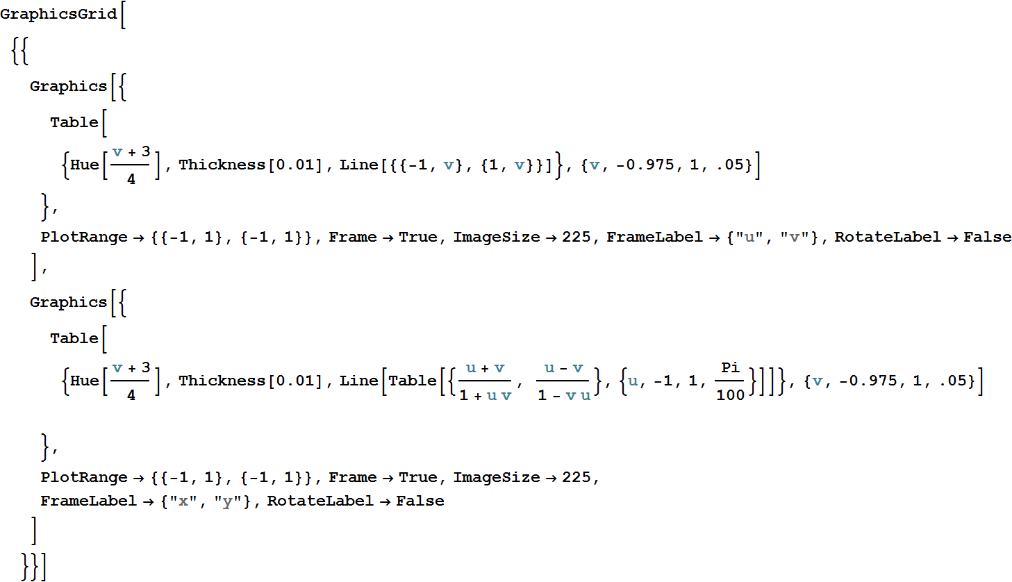
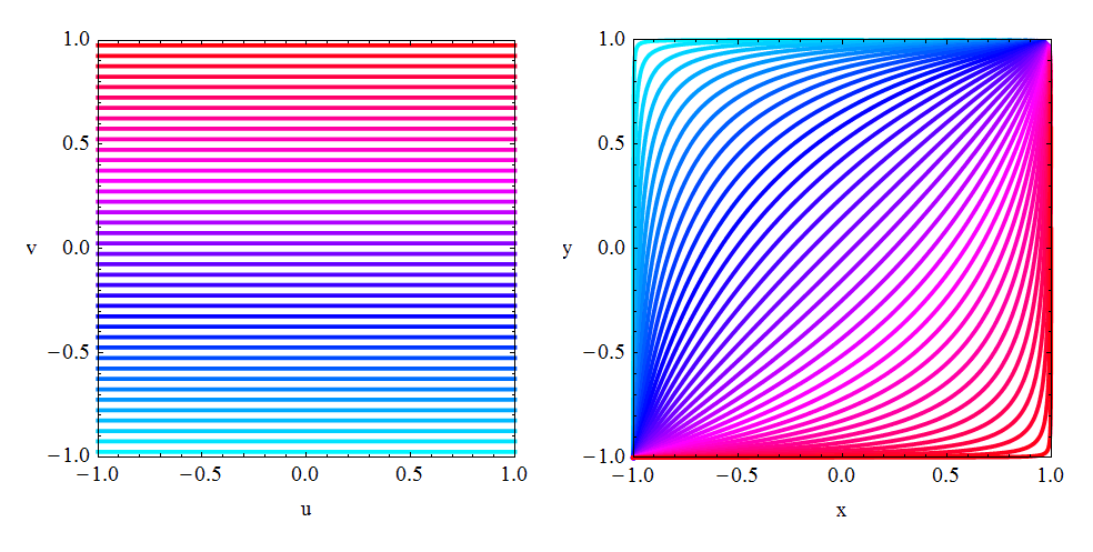
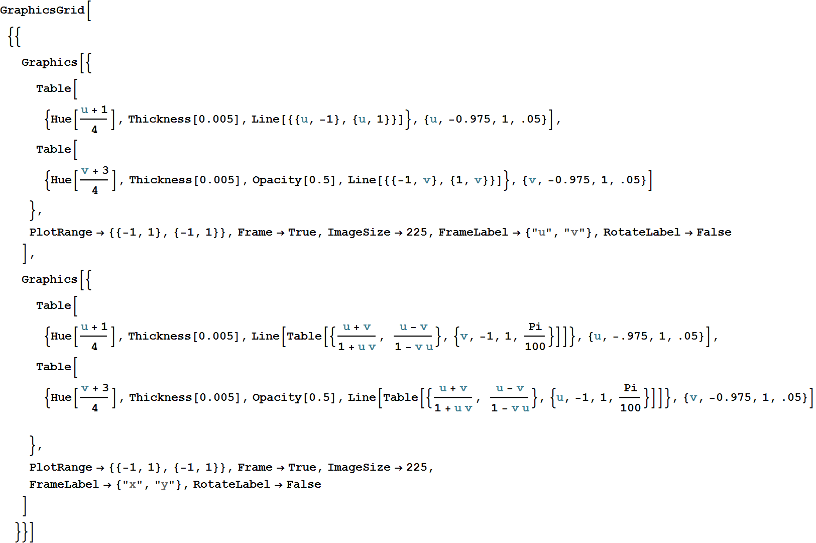
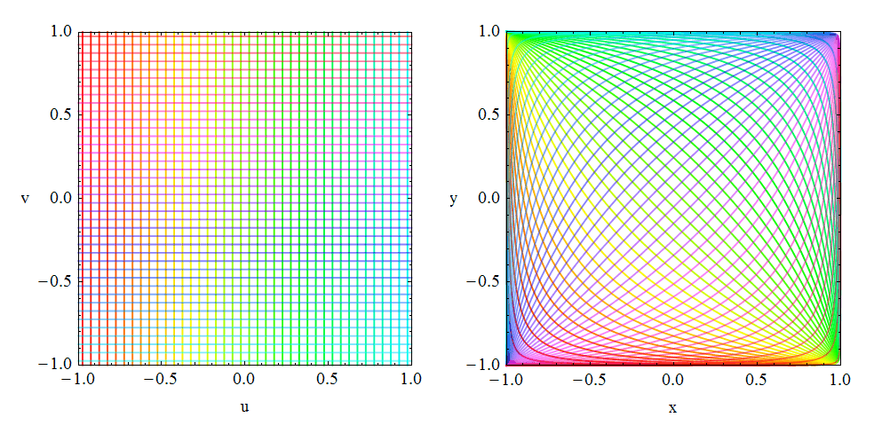
One way to visualize this mapping is to plot the grid of coordinate lines in uv-plane and map them into curves in xy-plane. For example the line u=1/2 is being mapped into the curve { }
}
In[76]:=
Out[76]=
In[77]:=
Out[77]=
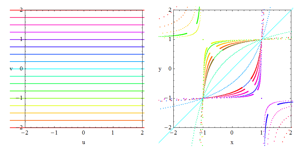
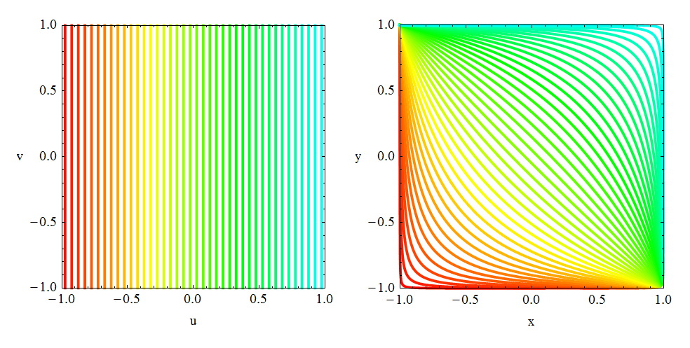
Since we see some overlap it is clear that we will have to narrow down the area in uv-plane.
In[78]:=

Out[78]=
In[79]:=
Out[79]=
In[80]:=
Out[80]=
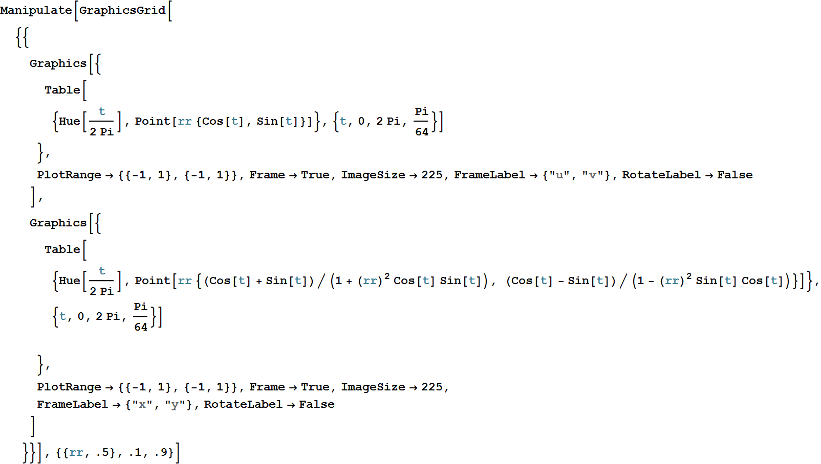
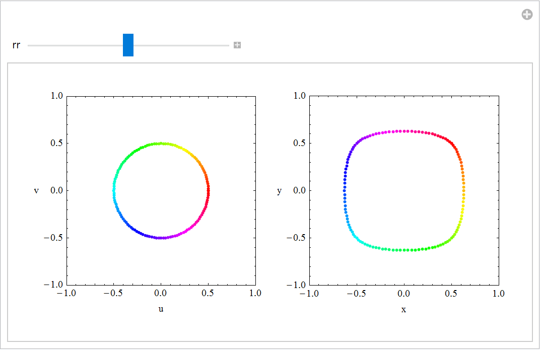
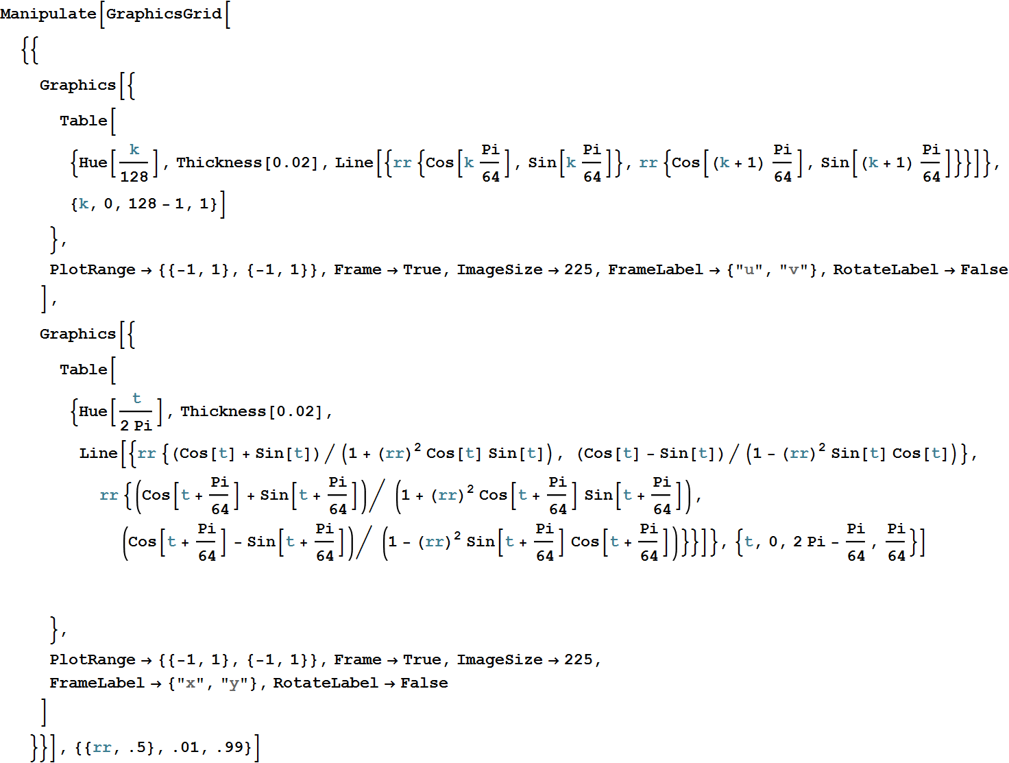
Just for fun
In[81]:=
Out[81]=
In[82]:=
Out[82]=
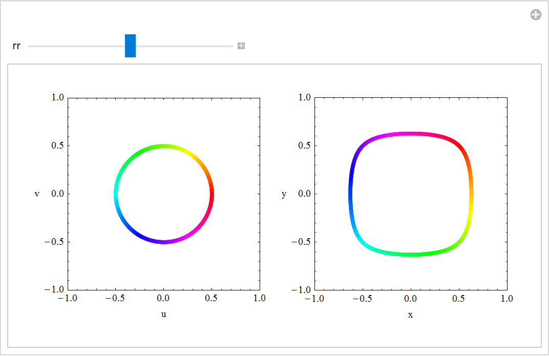
Let us go back to the change of variables:
![]()
This is how Mathematica calculates the Jacobian matrix:
In[83]:=

Out[83]=

We need the determinant of the Jacobian matrix
In[84]:=

Out[84]=

We notice that this quantity is negative for u, v being in [-1,1]. So the absolute value is
In[85]:=

Out[85]=

We need to understand which set in uv-plane is being mapped onto the unit square with vertices (0,0), (1,0), (1,1), (1,0) in xy-plane.
Next we list points in uv-plane and their images in xy-plane
(0,0) goes to (0,0)
(1,1) goes to (1,0)
(1,-1) goes to (0,1)
(1,0) goes to (1,1)
This indicates that the triangle with vertices (0,0), (1,-1), (1,1) is being mapped onto the unit square. The following graphics confirms that.
In[86]:=
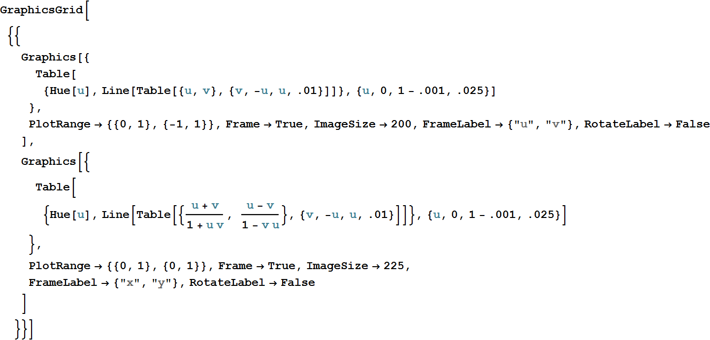
Out[86]=
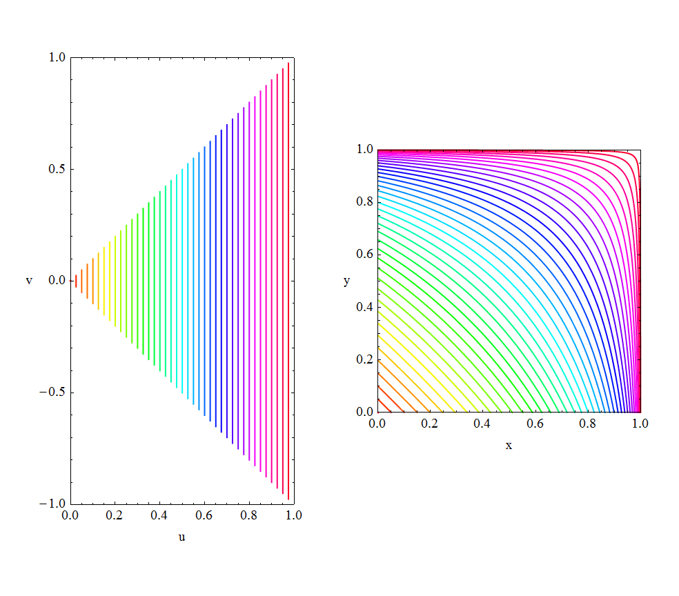
Now we substitute the new variables into the integrand
In[87]:=

Out[87]=

We notice that this quantity is positive. This expression needs to be multiplied by the absolute value of the determinant of the Jacobian matrix. Thus, the new integrand is
In[88]:=

Out[88]=

So, we need to calculate the integral

This integral is easily calculable by hand. However, for efficiency I do it in Mathematica here.
In[89]:=

Out[89]=

Now we integrate with respect to u. This is also a simple change of variables integral.
In[90]:=

Out[90]=
![]()
A famous triple integral
We consider the integral  .
.
Mathematica does calculate this integral.
In[91]:=

Out[91]=
![]()
Our goal is to understand this result using change of variables in double integral.
The change of variables here is

Good way to think about this change of variables is as a mapping from uvw-space into xyz-space.

This is how Mathematica calculates the Jacobian matrix:
In[92]:=

Out[92]=
![]()
We need the determinant of the Jacobian matrix
In[93]:=

Out[93]=
![]()
This function is always positive. So, no problems here.
We need to understand which set in uv-plane is being mapped onto the unit cube with the vertices (0,0,0), (1,0,0), (1,1,0), (1,0,0), (0,0,1), (1,0,1), (1,1,1), (1,0,1) in xyz-space.
Next we list points in uvw-space and their images in xyz-space
(0,0,0) goes to (0,0,0)
(![]() ,0,0) goes to (1,0,0)
,0,0) goes to (1,0,0)
(0,![]() ,0) goes to (0,1,0)
,0) goes to (0,1,0)
(0,0,![]() ) goes to (0,0,1)
) goes to (0,0,1)
(![]() ,
,![]() ,
,![]() ) goes to (1,1,1)
) goes to (1,1,1)
This indicates that the polytope with vertices (0,0,0), (![]() ,0,0), (0,
,0,0), (0,![]() ,0), (0,0,
,0), (0,0,![]() ,0), (
,0), (![]() ,
,![]() ,
,![]() ) is being mapped onto the unit cube. Our next goal is to confirm that. Here is the image of the polytope:
) is being mapped onto the unit cube. Our next goal is to confirm that. Here is the image of the polytope:
In[94]:=

Out[94]=
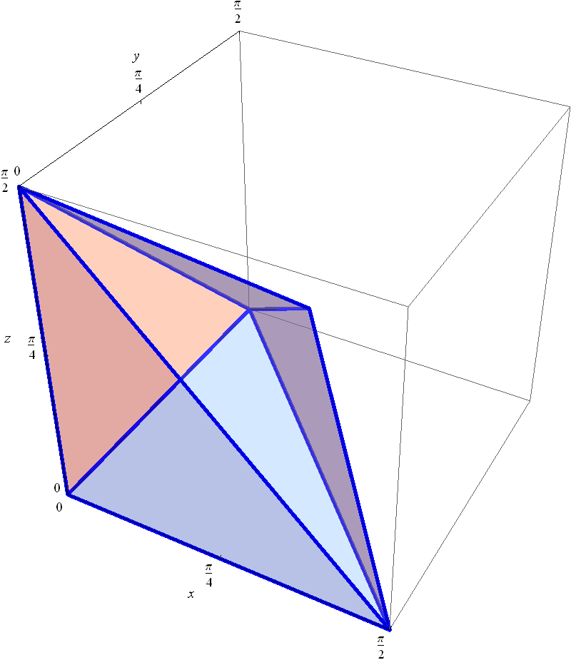
This polytope can be described mathematically as
![]()
Mathematica can plot this polytope using these inequalities:
In[95]:=

Out[95]=
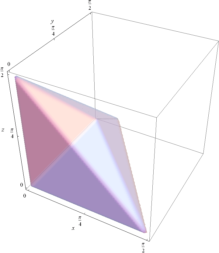
Next we will use Manipulate to slice this polytope into triangles which we will map into the unit cube.
In[96]:=
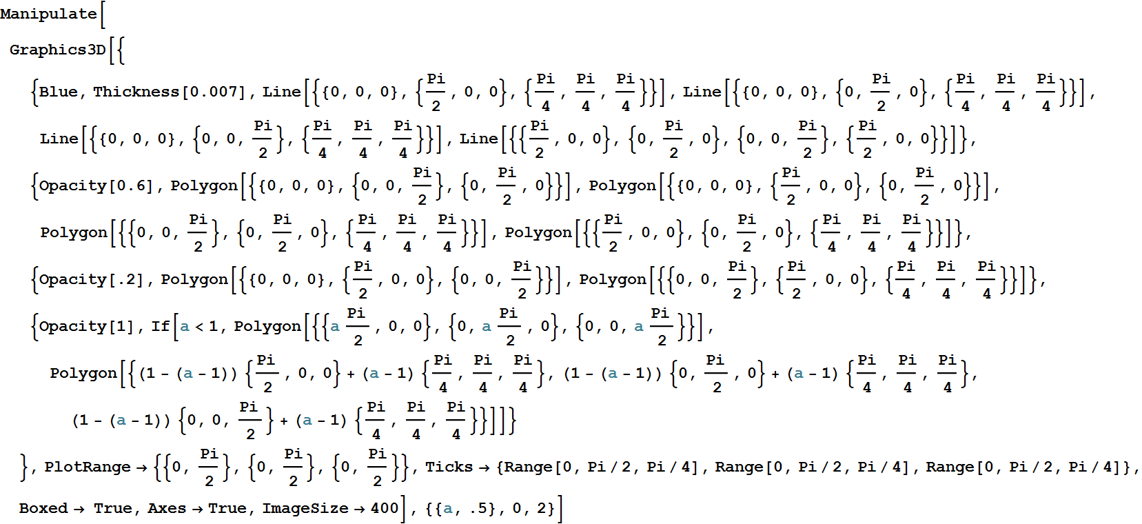
Out[96]=
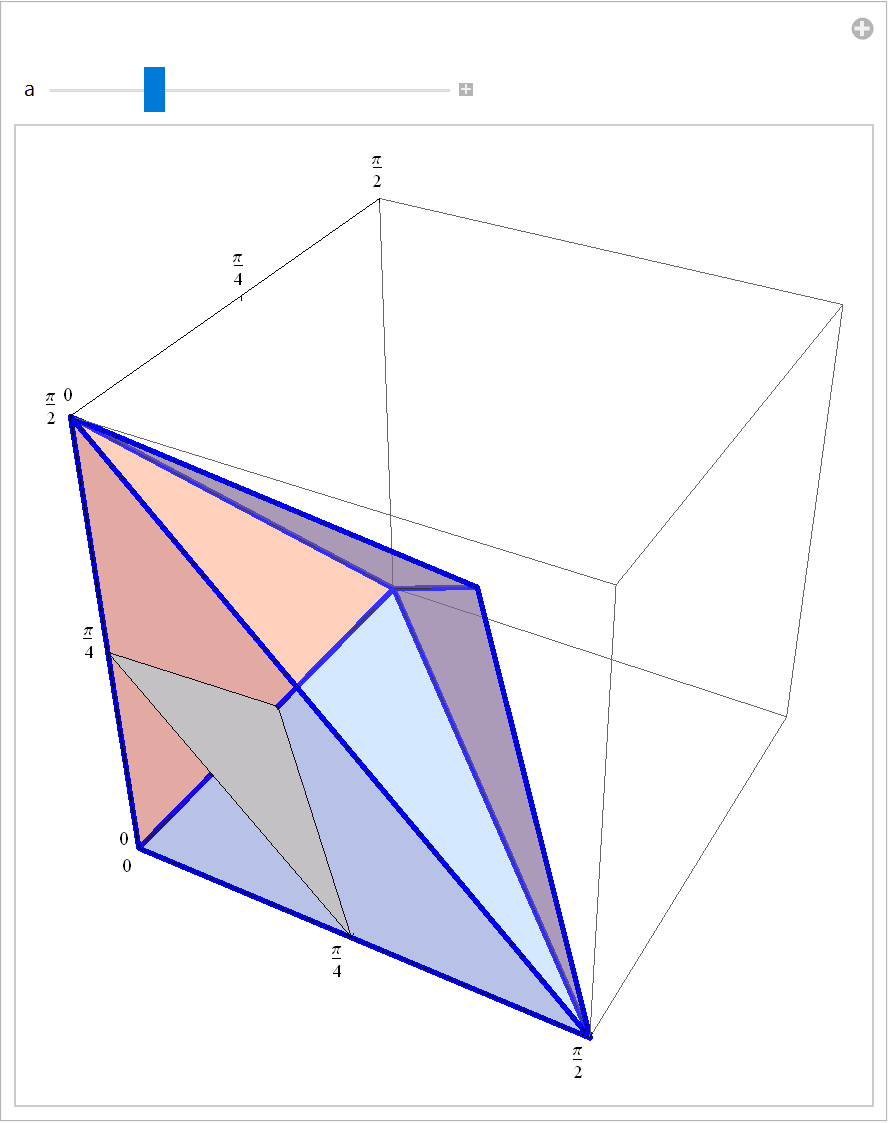
In the above Manipulation I used Polygon command to draw the slicing triangles. For that I needed only the vertices of the triangles. However, to map the triangles into xyz-space I need to represent the triangles using two parameters s and t. How to do that?
If we have two points say A and B, then all the point on the line segment AB are given by (1-s) A + s B where 0 ≤ s ≤1 .
We use the same idea for three points, say A, B, C. First we represent all the points on the line segments AB and AC
(1-s) A + s B, 0 ≤ s ≤1 and (1-s) A + s C, 0 ≤ s ≤1 .
Now for a fixed s I use parameter t to represent all the point on the line segment connecting the point
(1-s) A + s B and (1-s) A + s C :
(1-t)((1-s) A + s B) + t ((1-s) A + s C) where 0 ≤ s, t ≤1 .
Simplifying the last expression we get the following formula for the surface of the triangle with vertices A, B, C
In[97]:=
![]()
Out[97]=
![]()
Thus the formula
(1-s)A +s (1-t) B + s t C where 0 ≤ s, t ≤1
represents the surface of the triangle with vertices A, B, C. I will illustrate this with a graphics:
In[98]:=
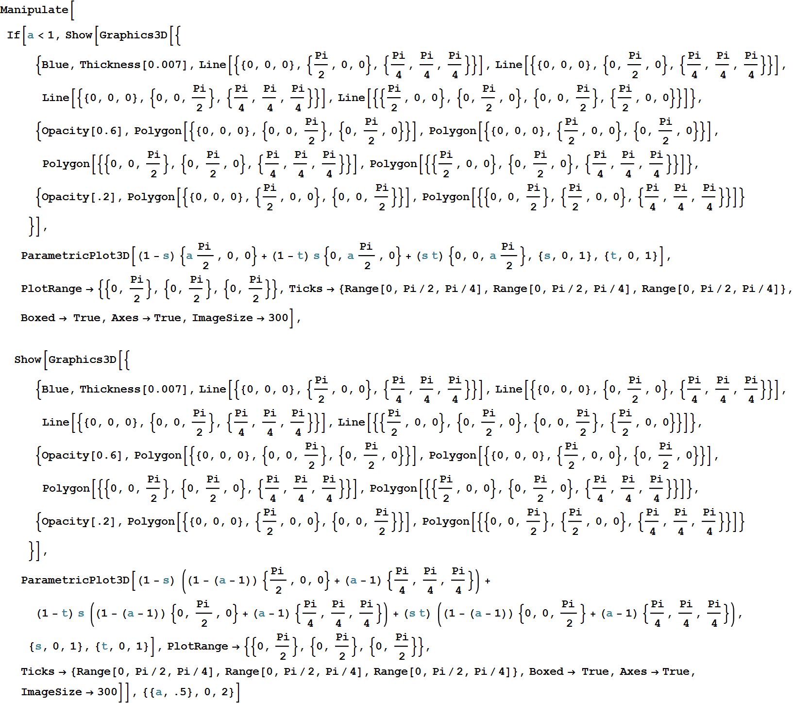
Out[98]=
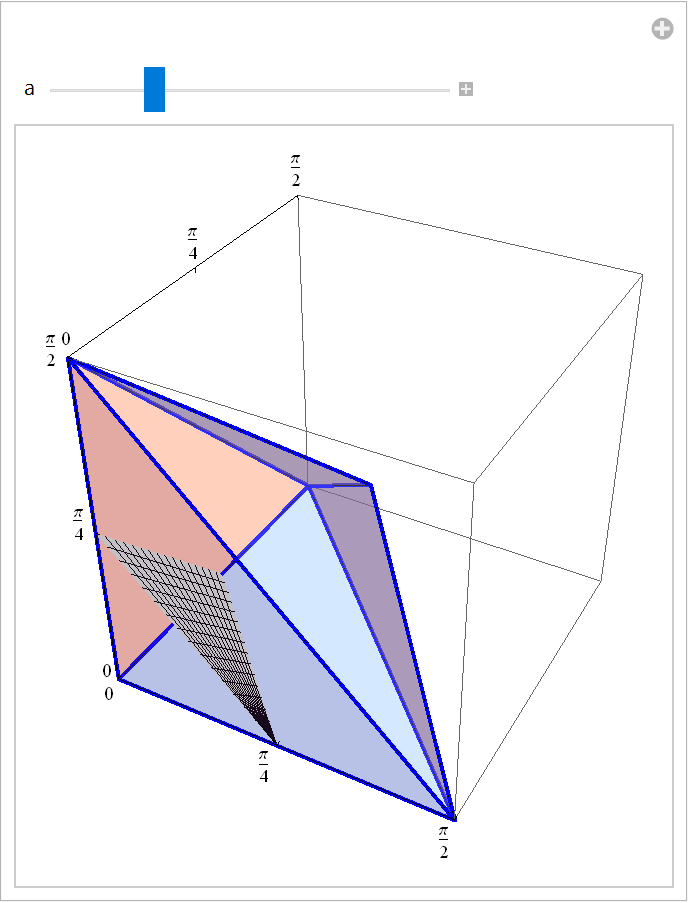
Next I use the mapping

In[99]:=

Out[99]=
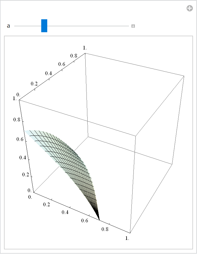
In[100]:=
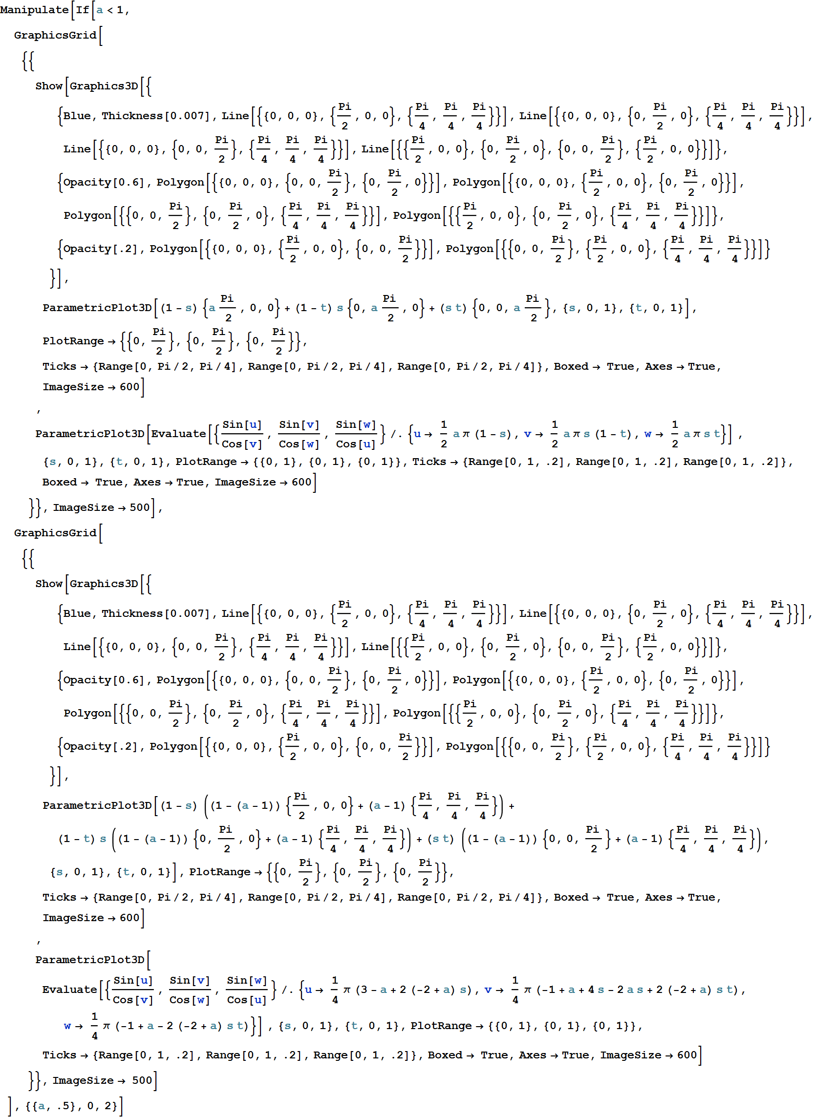
Out[100]=
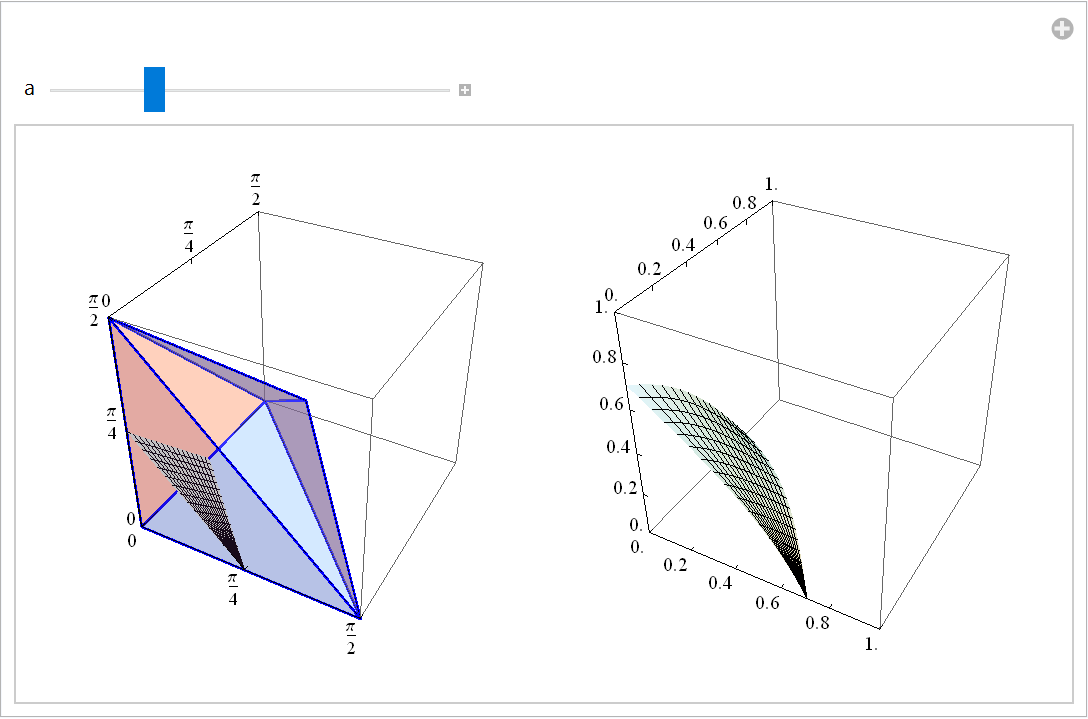
Now we substitute the new variables into the integrand
In[101]:=

Out[101]=

This expression needs to be multiplied by the absolute value of the determinant of the Jacobian matrix. Thus, the new integrand is
In[102]:=

Out[102]=
![]()
Thus, the integral is simply the volume of the polytope that found.
To calculate the volume of the polytope we split it into two pyramids.
One pyramid has vertices (0,0,0), ![]() ,
, ![]() ,
, ![]() . The base of this pyramid is equilateral triangle with the vertices
. The base of this pyramid is equilateral triangle with the vertices ![]() ,
, ![]() ,
, ![]() and the height of this pyramid is the line segment with the endpoints (0,0,0),
and the height of this pyramid is the line segment with the endpoints (0,0,0), ![]() . Thus the volume of this pyramid is
. Thus the volume of this pyramid is

One pyramid has vertices (0,0,0), ![]() ,
, ![]() ,
, ![]() ,
, ![]() . The base of this pyramid is equilateral triangle with the vertices
. The base of this pyramid is equilateral triangle with the vertices ![]() ,
, ![]() ,
, ![]() and the height of this pyramid is the line segment with the endpoints
and the height of this pyramid is the line segment with the endpoints ![]() ,
, ![]() . Thus the volume of this pyramid is
. Thus the volume of this pyramid is

Thus the volume of the polytope is

Problem 2. Your task
Calculate the famous double integral by using a change of variables similar to what was used to calculate the famous triple integral. Provide all the illustrations as I did in my calculation of the famous double integral.
Problem 3. Cissoid of Diocles
Prolog to Cissoid of Diocles problem
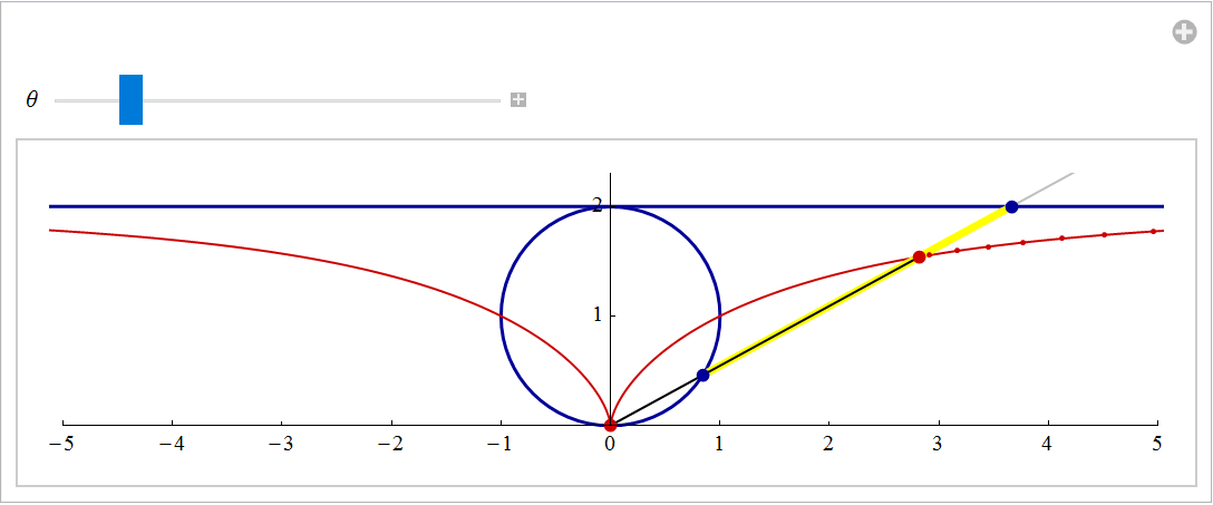
This problem is about the curve called Cissoid of Diocles. In fact this is a family of curves. Below is the construction of the Cissoid of Diocles based on circle with radius one.
In[103]:=
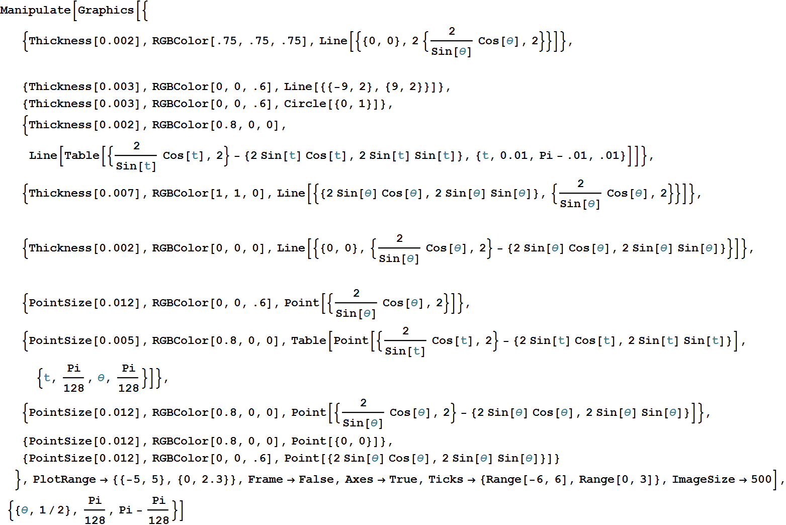
Out[103]=
Your task
Learn about the Cissoid of Diocles family of curves. The corresponding Wikipedia page is very informative. Based on that information answer the following two questions:
Length
Calculate the length of the part of the Cissoid of Diocles which is inside the circle which is used in the definition of that Cissoid. That is the maroon length in the picture below.
In[104]:=

Out[104]=
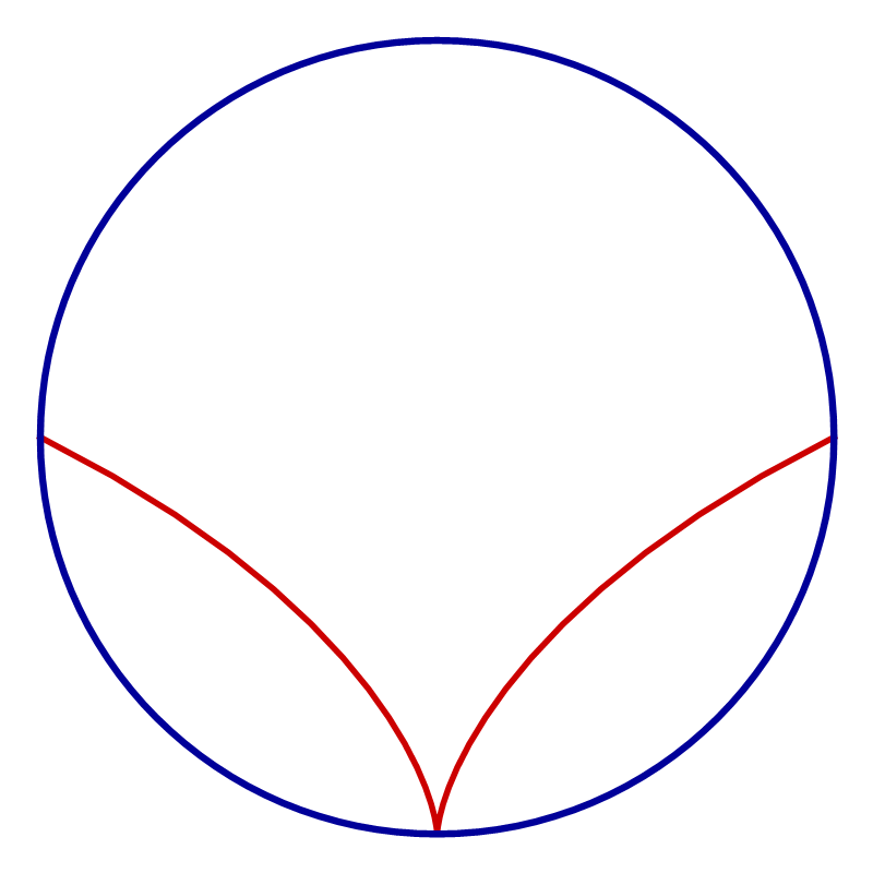
In your response to this question you should present and illustrate all the relevant information that you found on the Internet. You should present at least two distinct calculations for the length. The exact value for the length is expected.
Area
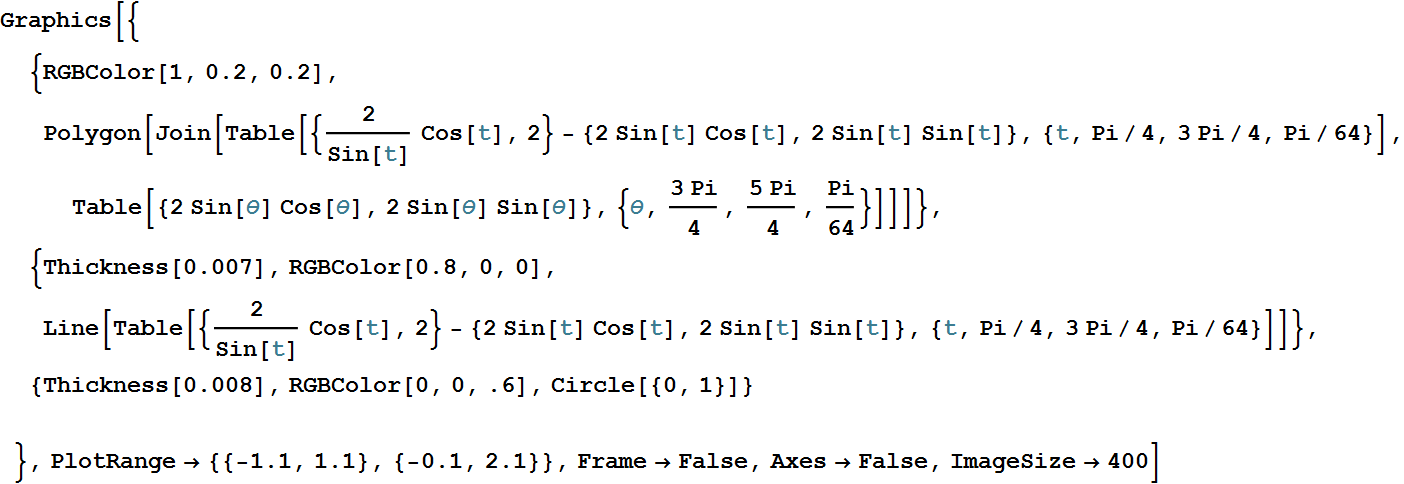
Calculate the area which is below the Cissoid of Diocles and which is inside the circle which is used in the definition of that Cissoid. That is the red area in the picture below.
In[105]:=
Out[105]=
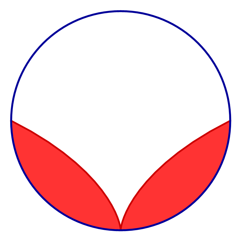
In your response to this question you should present and illustrate all the relevant information that you found on the Internet. You should present at least two distinct calculations for the area. The exact value for the area is expected .
Problem 4. Explore Ellipses
Let a and b be positive real numbers. Consider the ellipse

The parametric equation for this ellipse is
![]()
In this problem we consider only the ellipses in this canonical form.
Area
Calculate
Present at least three different ways to evaluate the area enclosed by this ellipse.
Together
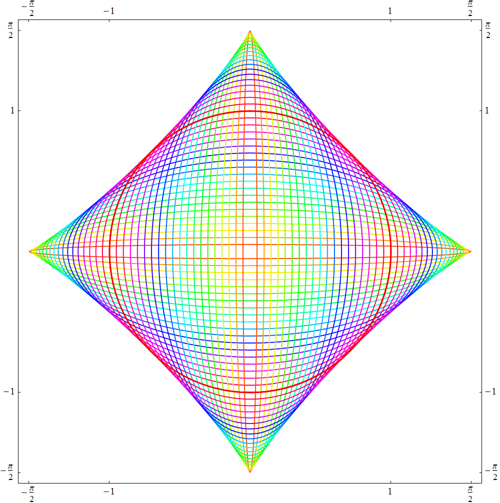
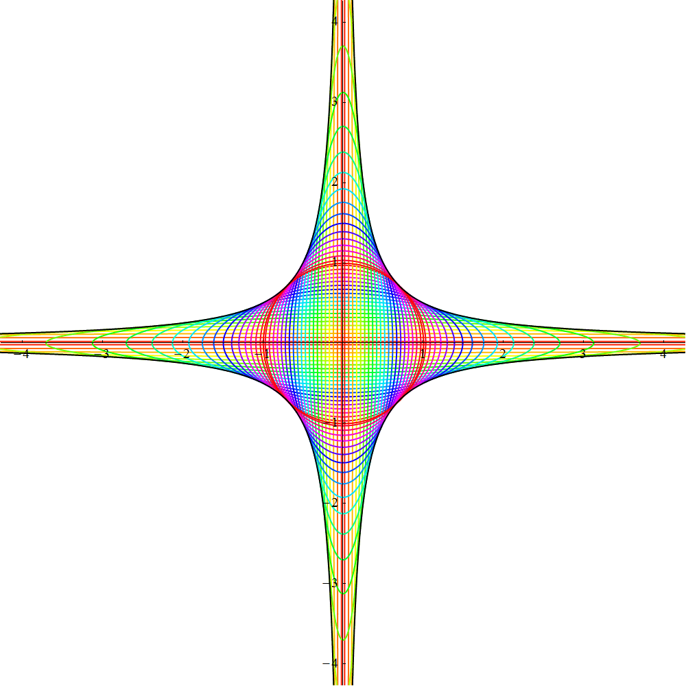
The most famous circle is the unit circle. The area enclosed by the unit circle is π. Determine the family of all ellipses each one of which encloses the area π. Replicate the picture below which shows 40 such ellipses.
Length
Calculate
Determine the exact formula for the circumference of the ellipse introduced in the introduction to this problem. Determine at least three different, but equivalent, ways of writing this formula. Give explanations of the functions that you are using.
Together
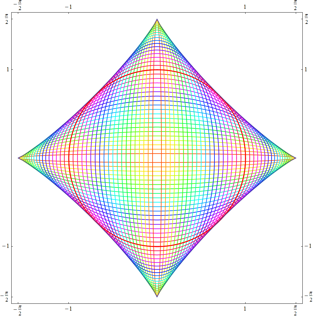
The most famous circle is the unit circle. The the circumference of the unit circle is 2π. Determine the family of all ellipses each one of which has the circumference 2π. Replicate the picture below which shows 40 such ellipses.
