-
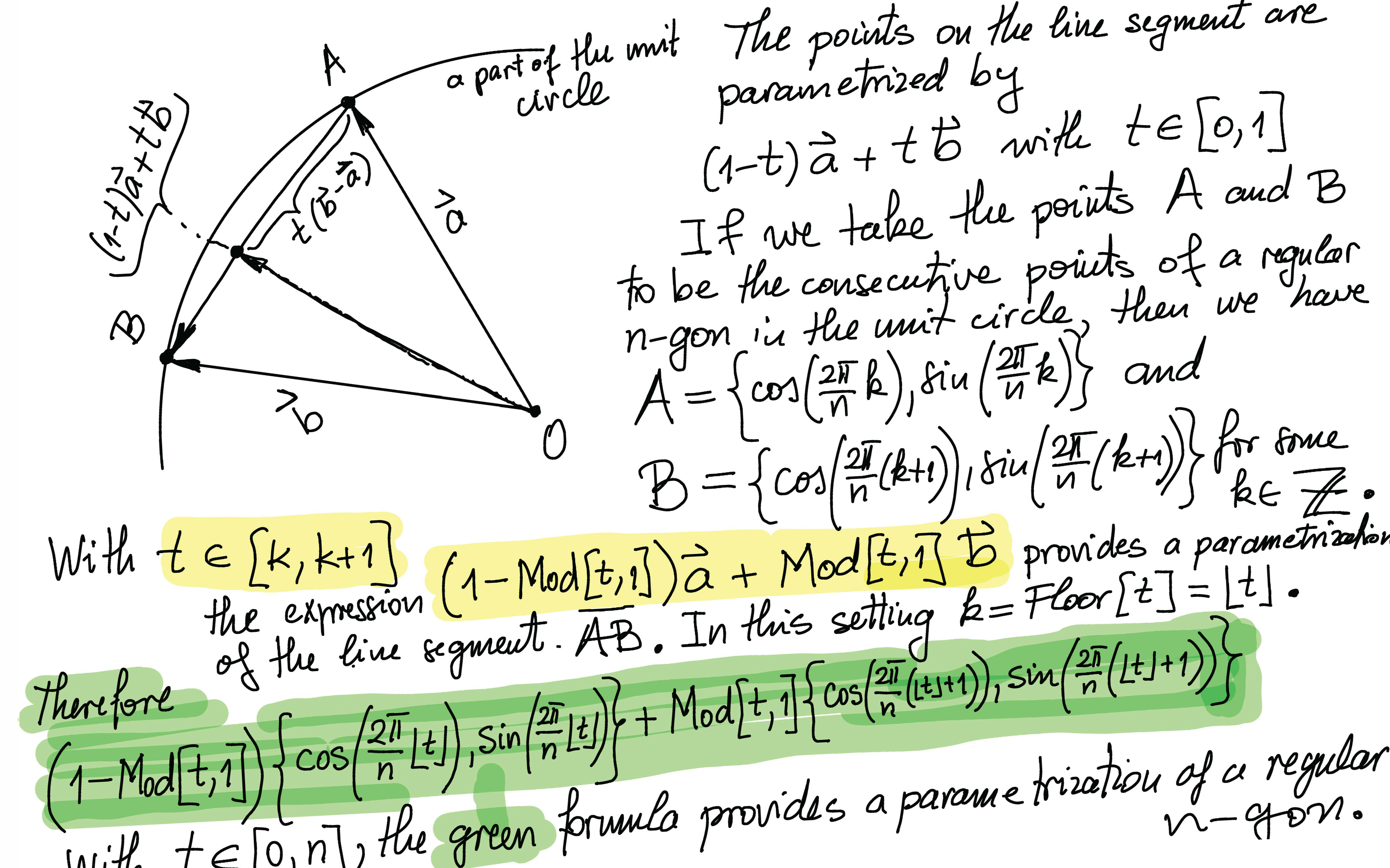
On Thursday and Friday we explored an amazing function
\[
\forall\mkern 1mu x \in \mathbb{R} \qquad x \mapsto \frac{\sin (x)+\tanh (x)}{1 + \sin (x) \tanh (x)}.
\]
In the Mathematica code below, I will consistently write this function as a pure function:
(Sin[#] + Tanh[#])/(1 + Sin[#] Tanh[#]) &
I find this preferable to assigning it a name, since it keeps us constantly aware of the function's spirit: Sin[#]& and Tanh[#]&.
-
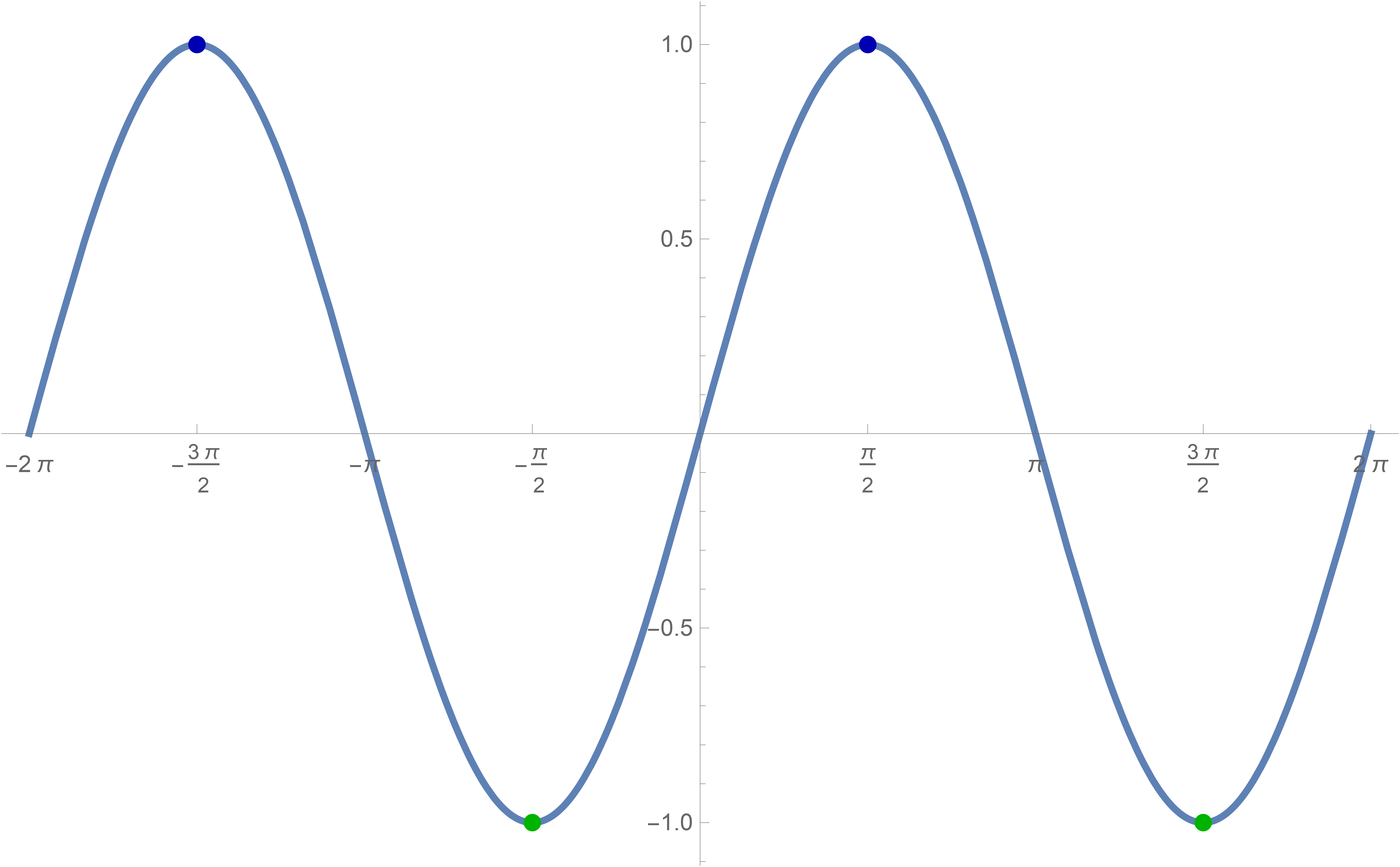
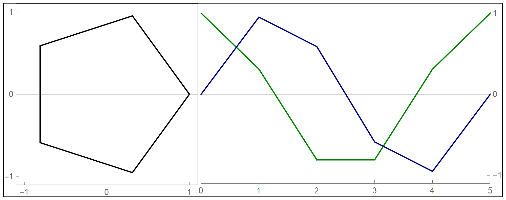
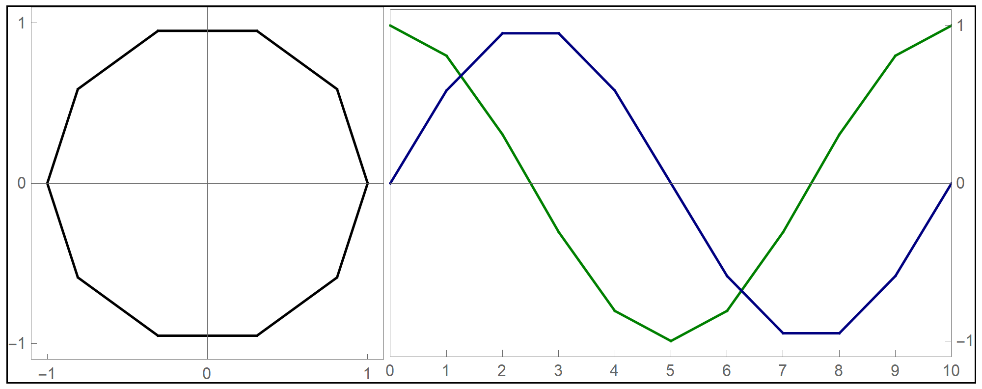
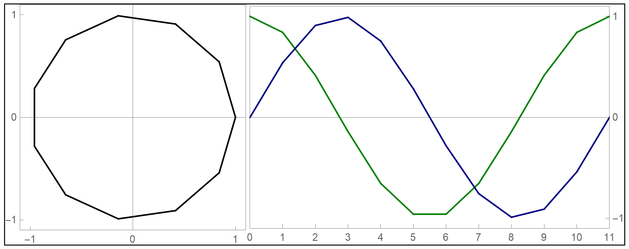
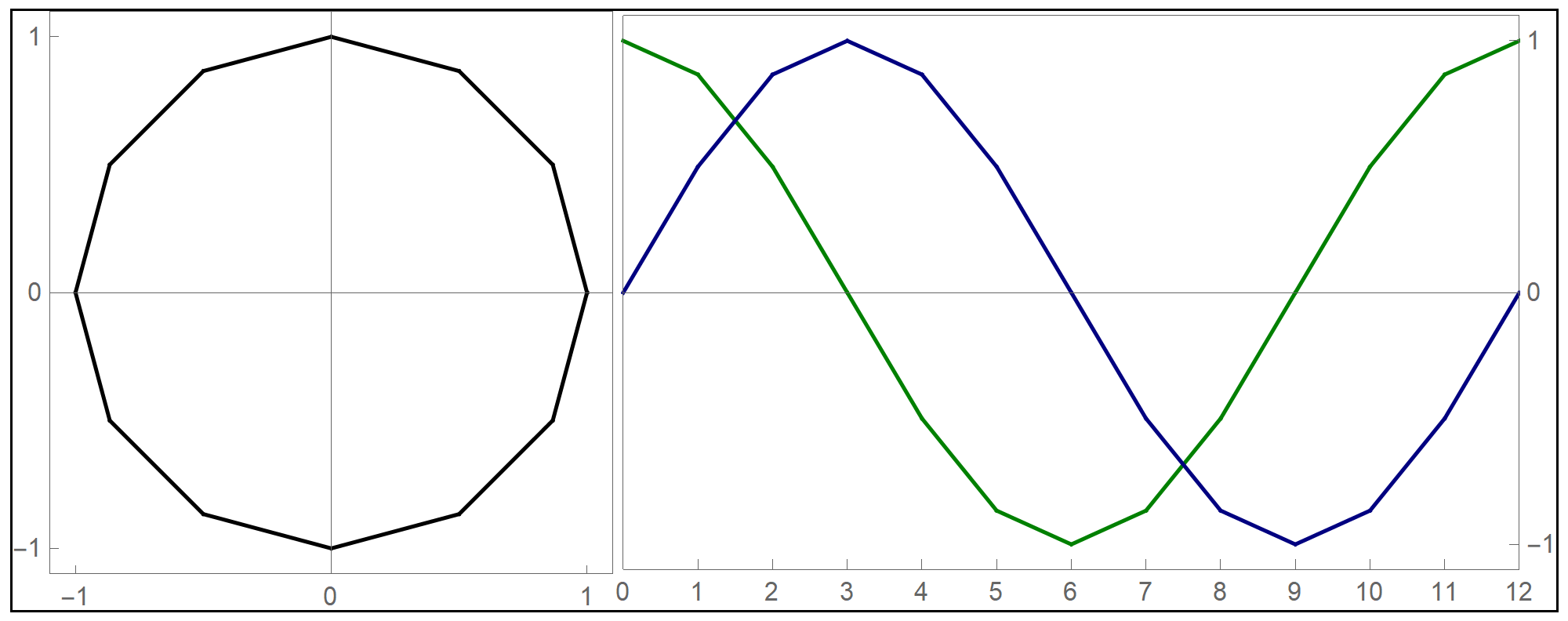
Before preceding with the explorations of the given function, let us review what we know about its components
Plot[Sin[#] &[x], {x, -2 Pi, 2 Pi}, PlotStyle -> {Thickness[0.005]},
 Epilog -> {{PointSize[0.0125], RGBColor[0.7 {0, 0, 1}],
    Point[{#, Sin[#]}] & /@
     Range[-4 Pi + Pi/2, 4 Pi, 2 Pi]}, {PointSize[0.0125],
    RGBColor[0.7 {0, 1, 0}],
    Point[{#, Sin[#]}] & /@ Range[-4 Pi + (3 Pi)/2, 4 Pi, 2 Pi]}},
 Ticks -> {Range[-4 Pi, 4 Pi, Pi/2], Automatic}]
Plot[Tanh[#] &[x], {x, -8, 8}, PlotStyle -> {Thickness[0.005]},
 Epilog -> {{Thickness[0.003], RGBColor[0.7 {0, 0, 1}],
    Line[{{{-10, 1}, {10, 1}}}]}, {Thickness[0.003],
    RGBColor[0.7 {0, 1, 0}], Line[{{{-10, -1}, {10, -1}}}]}},
 Ticks -> {Range[-10, 10, 1], Automatic}]
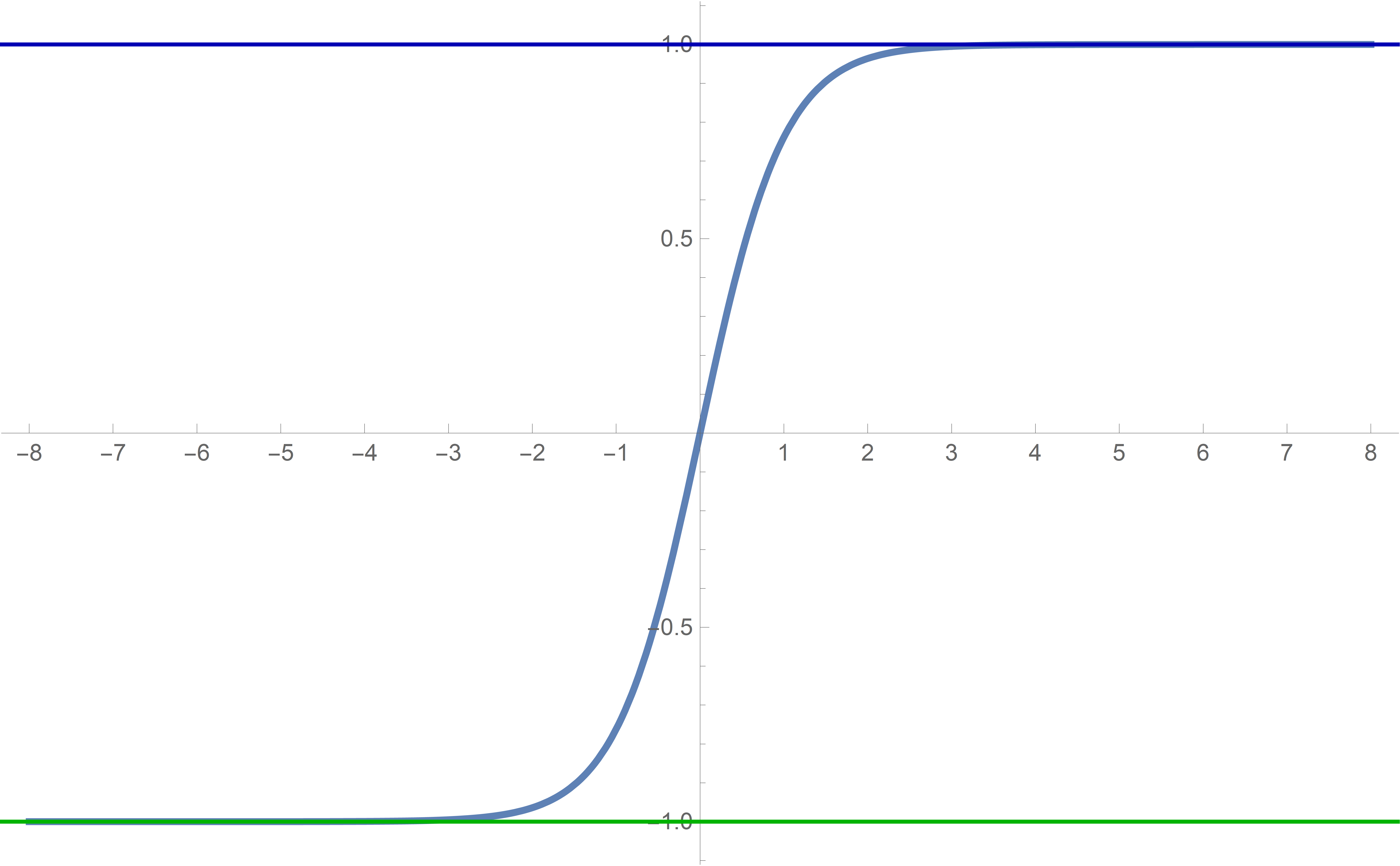
We see that Tanh[#]& is an odd sigmoid function with the horizontal asymptotes at \(y=1\) and \(y=-1\) and that Tanh[#]& approaches the asymptotes very rapidly. In fact
\begin{align*}
\tanh(20) &\approx 0.99999999999999999150329148941682204543855819119099\\
\tanh(50) &\approx 0.99999999999999999999999999999999999999999992559848
\end{align*}
-
A basic Plot[...] results in
Plot[(Sin[#] + Tanh[#])/(1 + Sin[#] Tanh[#])&[x], {x, -9, 9}, PlotStyle -> {Thickness[0.005]}]
The graph indicates that the function is odd:
\[
\forall\mkern 1mu x \in \mathbb{R} \quad \frac{\sin (-x)+\tanh (-x)}{1 + \sin (-x) \tanh (-x)} = \frac{-\sin (x)-\tanh (x)}{1 + \sin (x) \tanh (x)} = - \frac{\sin (x)+\tanh (x)}{1 + \sin (x) \tanh (x)}
\]
Thus for all the features we can focus on the positive real numbers.
-
Natural questions arise: Is this function defined for all real numbers? What is the exact range of this function?
-
To understand this function we have to use our knowledge of its components Sin[#]& and Tanh[#]&.
We know that
Sin[#] & /@ Range[-10 Pi + Pi/2, 10 Pi, 2 Pi]
will result in all 1s. While
Sin[#] & /@ Range[-10 Pi + 3 Pi/2, 10 Pi, 2 Pi]
will result in all -1s.
Therefore it is interesting to evaluate our given function at those values. And we can do that "on paper". For every integer \(k\) we have
\[
\frac{\sin \bigl(\tfrac{\pi}{2}+2 k \pi\bigr)+\tanh(\tfrac{\pi}{2}+2 k \pi\bigr)}{1 + \sin(\tfrac{\pi}{2}+2 k \pi\bigr) \tanh(\tfrac{\pi}{2}+2 k \pi\bigr)}
= \frac{1+\tanh(\tfrac{\pi}{2}+2 k \pi\bigr)}{1 + 1 \tanh(\tfrac{\pi}{2}+2 k \pi\bigr)}
= \Large 1
\]
and
\[
\frac{\sin \bigl(\tfrac{3\pi}{2}+2 k \pi\bigr)+\tanh(\tfrac{3\pi}{2}+2 k \pi\bigr)}{1 + \sin(\tfrac{3\pi}{2}+2 k \pi\bigr) \tanh(\tfrac{3\pi}{2}+2 k \pi\bigr)}
= \frac{-1+\tanh(\tfrac{\pi}{2}+2 k \pi\bigr)}{1 + (-1) \tanh(\tfrac{\pi}{2}+2 k \pi\bigr)}
= - \Large 1
\]
There is a warning in the denominator of the last expression
\[
1 + (-1) \tanh(\tfrac{\pi}{2}+2 k \pi\bigr) = 1 - \tanh(\tfrac{\pi}{2}+2 k \pi\bigr).
\]
We have seen earlier that \(\tanh(50)\) is very close to \(1\). So when the positive integer \(k\) is large, \(\tanh(\tfrac{\pi}{2}+2 k \pi\bigr)\) is very close to \(0\). It can be so close to \(0\) that Mathematica can mistakenly take it to be \(0\). We need to be aware of this in out calculations.
-
Let us implement what we calculated in the preceding item on a graph of the given function.
Plot[(Sin[#] + Tanh[#])/(1 + Sin[#] Tanh[#]) &[x], {x, 0, 30},
 PlotStyle -> {Thickness[0.005]},
 Epilog -> {{PointSize[0.0125], RGBColor[0.7 {0, 0, 1}],
    Point[{#, (Sin[#] + Tanh[#])/(1 + Sin[#] Tanh[#])}] & /@
     Range[-4 Pi + Pi/2, 40 Pi, 2 Pi]}, {PointSize[0.0125],
    RGBColor[0.7 {0, 1, 0}],
    Point[{#,
        FullSimplify[(Sin[#] + Tanh[#])/(1 + Sin[#] Tanh[#])]}] & /@
     Range[-4 Pi + (3 Pi)/2, 40 Pi, 2 Pi]}},
 PlotRange -> {{0, 30}, {-1.1, 1.1}},
 Ticks -> {Range[-4 Pi, 40 Pi, Pi/2], Automatic}]
This graph clearly indicates that something suspicious is going on with this graph. What is happening near the \(x\)-values \(\dfrac{3\pi}{2}+2 k \pi\) for nonnegative values of the integer \(k\)?
This needs additional explorations.
-
I decided that it will be a good idea to zoom in near the \(x\)-values
\[
\dfrac{3\pi}{2}, \quad \dfrac{3\pi}{2}+2 \pi, \quad \dfrac{3\pi}{2}+4 \pi, \quad \dfrac{3\pi}{2}+6 \pi, \ldots
\]
To automate this process, I introduced the variable nn for the number of \(2\pi\) that I am adding and the variable dx for the range of the variable \(x\) that I am allowing. So, I graph the given function on the interval
{x, 2 nn Pi + (3 Pi)/2 - dx, 2 nn Pi + (3 Pi)/2 + dx}
I choose the following PlotRange->
PlotRange ->
{{2 nn Pi + (3 Pi)/2 - dx,  2 nn Pi + (3 Pi)/2 + dx}, {-1.1, 1.1}}
In the command below I use Module[] to make the variables nn and dx local.
Module[{nn, dx}, nn = 1; dx = (3/2) 10^(-4);
 Plot[(Sin[#] + Tanh[#])/(1 + Sin[#] Tanh[#]) &[x] , {x,
   2 nn Pi + (3 Pi)/2 - dx, 2 nn Pi + (3 Pi)/2 + dx},
  PlotPoints -> 1500, PlotStyle -> {Thickness[0.005]},
  PlotRange -> {{2 nn Pi + (3 Pi)/2 - dx,
     2 nn Pi + (3 Pi)/2 + dx}, {-1.1, 1.1}},
  Epilog -> {{Text[
      2 nn Pi + (3 Pi)/2, {2 nn Pi + (3 Pi)/2, 0.15}]}, {PointSize[
      0.01], RGBColor[0, 0.6, 0],
     Point[{#, -1}] & /@
      Range[2 (nn - 1) Pi + (3 Pi)/2, 2 (nn + 1) Pi + (3 Pi)/2,
       2 Pi]}}, Axes -> True,
  Ticks -> {{#, N[#]} & /@
     Range[2 nn Pi + (3 Pi)/2 - dx, 2 nn Pi + (3 Pi)/2 + dx, dx/4],
    Automatic}, ImageSize -> 800]]
Module[{nn, dx}, nn = 2; dx = (3/2) 10^(-6);
 Plot[(Sin[#] + Tanh[#])/(1 + Sin[#] Tanh[#]) &[x] ,
  {x, 2 nn Pi + (3 Pi)/2 - dx, 2 nn Pi + (3 Pi)/2 + dx},
  PlotPoints -> 1500, PlotStyle -> {Thickness[0.005]},
  PlotRange -> {{2 nn Pi + (3 Pi)/2 - dx,
     2 nn Pi + (3 Pi)/2 + dx}, {-1.1, 1.1}},
  Epilog -> {{Text[
      2 nn Pi + (3 Pi)/2, {2 nn Pi + (3 Pi)/2, 0.15}]}, {PointSize[
      0.01], RGBColor[0, 0.6, 0],
     Point[{#, -1}] & /@
      Range[2 (nn - 1) Pi + (3 Pi)/2, 2 (nn + 1) Pi + (3 Pi)/2,
       2 Pi]}}, Axes -> True,
  Ticks -> {{#, N[#]} & /@
     Range[2 nn Pi + (3 Pi)/2 - dx, 2 nn Pi + (3 Pi)/2 + dx, dx/4],
    Automatic}, ImageSize -> 800]]
Module[{nn, dx}, nn = 3; dx = (3/2) 10^(-8);
 Plot[(Sin[#] + Tanh[#])/(1 + Sin[#] Tanh[#])&[x],
 {x, 2 nn Pi + (3 Pi)/2 - dx, 2 nn Pi + (3 Pi)/2 + dx},
  PlotPoints -> 1500, PlotStyle -> {Thickness[0.005]},
  PlotRange -> {{2 nn Pi + (3 Pi)/2 - dx,
     2 nn Pi + (3 Pi)/2 + dx}, {-1.1, 1.1}},
  Epilog -> {
  {Text[2 nn Pi + (3 Pi)/2, {2 nn Pi + (3 Pi)/2, 0.15}]},
  {PointSize[0.01], RGBColor[0, 0.6, 0],
     Point[{#, -1}]&/@
 Range[2 (nn - 1) Pi + (3 Pi)/2, 2 (nn + 1) Pi + (3 Pi)/2, 2 Pi]}},
  Axes -> True, Ticks -> {{#, N[#]}&/@
     Range[2 nn Pi + (3 Pi)/2 - dx, 2 nn Pi + (3 Pi)/2 + dx, dx/4],
    Automatic}, ImageSize -> 800]]
But, unfortunately, this strategy does not work for nn = 3. The last graph above is not very informative. Even worse, when we zoom in to dx = (3/2) 10^(-9), Mathematica reports errors. I illustrate the errors just by numerical calculations below.
Module[{nn, dx}, nn = 3; dx = (3/2)*10^-(9);
 N[ (Sin[#] + Tanh[#])/(1 + Sin[#] Tanh[#])] & /@
  Range[2 nn Pi + (3 Pi)/2 - dx, 2 nn Pi + (3 Pi)/2 + dx, dx/4]]
Resulting in
But, by carefully considering our calculations above we understand the source for these errors. Mathematica thinks that it encounters zero in the denominator. It is possible that we overcome this problem if we increase the precision with which Mathematica does the calculations. We do that in the next item.
-
To overcome the calculational problem at the end of the preceding item, we use SetPrecision[].
Module[{nn, dx}, nn = 3; dx = (3/2)*10^-(9);
 N[SetPrecision[(Sin[#] + Tanh[#])/(1 + Sin[#] Tanh[#]), 100]] & /@
  Range[2 nn Pi + (3 Pi)/2 - dx, 2 nn Pi + (3 Pi)/2 + dx, dx/4]]
Resulting in

These numbers are not extreme. The extremely small numbers are in the denominator of the given function.
I was not able to use SetPrecision[] in Plot[]. A solution that I found is in the next item.
-
I decided to replace Plot[] with just ploting points on the graph of the given function in Graphics[]. Also, instead graphing the given function near
\[
\dfrac{3\pi}{2}, \quad \dfrac{3\pi}{2}+2 \pi, \quad \dfrac{3\pi}{2}+4 \pi, \quad \dfrac{3\pi}{2}+6 \pi,
\quad \ldots, \quad
\dfrac{3\pi}{2}+2 k \pi
\]
for large positive integers \(k\), I shift the function to the left, and plot the shifted function near \(0\); the shifted function being
\[
\forall\mkern 1mu x \in (-1, 1) \qquad
x \mapsto \frac{\sin\bigl(\delta x + \tfrac{3 \pi}{2} + 2 k \pi\bigr)
+ \tanh\bigl(\delta x + \tfrac{3 \pi}{2} + 2 k \pi\bigr)}
{1 + \sin\bigl(\delta x + \tfrac{3 \pi}{2} + 2 k \pi\bigr) \tanh\bigl(\delta x + \tfrac{3 \pi}{2} + 2 k \pi\bigr)}.
\]
Here I use \(\delta \gt 0\) instead of dx and \(k\) instead of nn for a nonnegative integer.
Module[{dx, pws, nn}, nn = 12;
 (* dx below is the small range of x, how small is given with the \
powers 10^(-1) from the list below  *)
 pws = {4, 7, 9, 12, 15, 17, 20, 23, 26, 28, 31, 34, 37, 39, 42, 45,
   47, 50, 53, 56, 58, 61, 64, 67, 69, 72, 75, 77, 80, 83, 86, 88, 91,
    94, 96, 99, 102, 105, 107, 110, 113, 116, 118, 121, 124, 126, 129,
    132, 135, 137};
 dx = 3/2*10^-pws[[nn]];
 Graphics[{
   (* Below are 201 points on the graph near the value 2nn Pi+(3 Pi)/
   2 *)

   {PointSize[0.005], RGBColor[0.37, 0.51, 0.71],
    Point[{#,
        SetPrecision[(
         Sin[dx # + (3 Pi)/2] + Tanh[dx # + 2 nn Pi + (3 Pi)/2])/(
         1 + Sin[dx # + (3 Pi)/2] Tanh[dx # + 2 nn Pi + (3 Pi)/2]),
         300]}] & /@ Range[-1, 1, (1/2)*10^(-2)]},
   (* Which point is considered is shown below,
   exact and approximate *)
    {Text[2 nn Pi + (3 Pi)/2, {0, 0.175}],
    Text[N[2 nn Pi + (3 Pi)/2, 4], {0, -0.08}]},

   (* below is the tickmark at the minimum shown *)
   {Thickness[0.003], Line[{{0, -0.015}, {0, 0.015}}]},
   (* the dark green minimum point of the function *)
   {PointSize[0.015], RGBColor[0.6 {0, 1, 0}], Point[{0, -1}]}
   },
  Axes -> True, AspectRatio -> 1/GoldenRatio,
  PlotRangePadding -> None, Frame -> False,
  Ticks -> {If[Abs[#] > 0.1, {#, (dx/3) #}, {#, ""}] & /@
     Range[-1, 1, 0.25], Automatic},
  PlotRange -> {{-1, 1}, {-1.1, 1.1}}, AxesOrigin -> {-1, 0},
  PlotLabel ->
   TableForm[{"nn =", nn}, TableDirections -> Row,
    TableSpacing -> 0.3], ImageSize -> 600]]
Click on the image below to see the zoomed graphs.
-
Finally, I want to calculate the \(x\)-intercepts near each minimum.
Module[{dx, pws, zxl, zxr, nn}, nn = 16;
 pws = {4, 7, 9, 12, 15, 17, 20, 23, 26, 28, 31, 34, 37, 39, 42, 45,
   47, 50, 53, 56, 58, 61, 64, 67, 69, 72, 75, 77, 80, 83, 86, 88, 91,
    94, 96, 99, 102, 105, 107, 110, 113, 116, 118, 121, 124, 126, 129,
    132, 135, 137};
 dx = 3/2*10^-pws[[nn]];
(* below we use FindRoot with Brent method to calculate the
x-intercepts first the left one then the right one *)
zxl = (x /. FindRoot[
     ff[x] == 0, {x, (3 Pi)/2 + 2 nn Pi - 1/1000, (3 Pi)/2 + 2 nn Pi},
      MaxIterations -> 2000, WorkingPrecision -> 200,
     Method -> "Brent"]);
 zxr = (x /.FindRoot[
     ff[x] == 0, {x, (3 Pi)/2 + 2 nn Pi, (3 Pi)/2 + 2 nn Pi + 1/1000},
      MaxIterations -> 2000, WorkingPrecision -> 200,
     Method -> "Brent"]);
 Graphics[{
   {PointSize[0.005], RGBColor[0.37, 0.51, 0.71],
    Point[{#,
        SetPrecision[(
         Sin[dx # + (3 Pi)/2] + Tanh[dx # + 2 nn Pi + (3 Pi)/2])/(
         1 + Sin[dx # + (3 Pi)/2] Tanh[dx # + 2 nn Pi + (3 Pi)/2]),
         300]}] & /@ Range[-1, 1, (1/2) 10^-2]},
   {PointSize[0.015], RGBColor[1, 0, 0],
    Point[{(zxl - ((3 Pi)/2 + 2 nn Pi))/dx , 0}],
    Point[{(zxr - ((3 Pi)/2 + 2 nn Pi))/dx , 0}]},
     {Text[2 nn Pi + (3 Pi)/2, {0, 0.175}],
    Text[N[2 nn Pi + (3 Pi)/2, 4], {0, -0.08}]}, {Thickness[0.003],
    Line[{{0, -0.015}, {0, 0.015}}]}, {PointSize[0.015],
    RGBColor[0, 0.6, 0], Point[{0, -1}]}
   },
  Axes -> True, AspectRatio -> 1/GoldenRatio,
  PlotRangePadding -> None, Frame -> False,
  Ticks -> {If[
       Abs[#] > 0.1, {#, ScientificForm[(dx/4) #, {3, 2}]}, {#,
        ""}] & /@ Range[-1, 1, 0.25], Automatic},
  PlotRange -> {{-1, 1}, {-1.1, 1.1}}, AxesOrigin -> {-1, 0},
  PlotLabel ->
   TableForm[{"nn =", nn}, TableDirections -> Row,
    TableSpacing -> 0.3], ImageSize -> 800]]
Click on the image below to see the zoomed graphs with the \(x\)-intercepts.


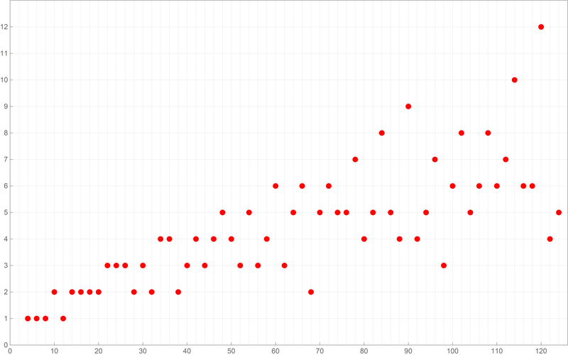
 Below is a colored plot of the first ten thousand values of the Goldbach lengths.
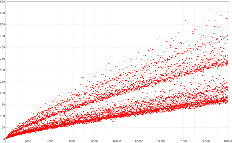
 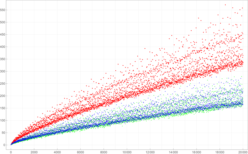 Below is a colored plot of the first fifty thousand values of the Goldbach lengths.
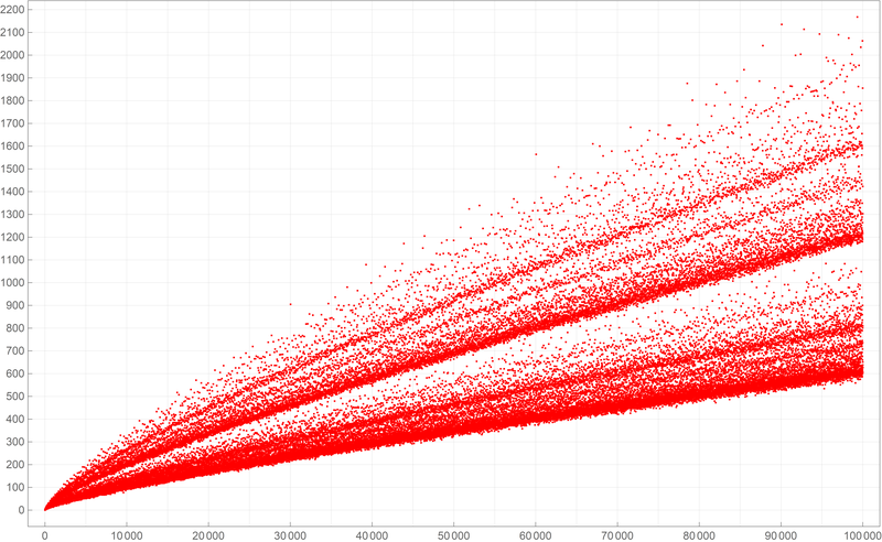
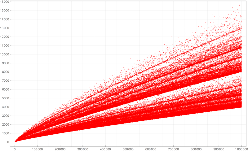
 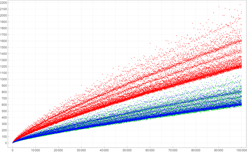 Below is a colored plot of the first five hundred thousand values of the Goldbach lengths. I wanted to create a colored version of the picture from Wikipedia.
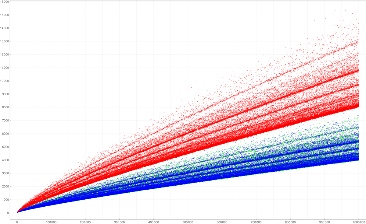


 The complete code for the above picture is
 Or, shortening the length of the touching line segments
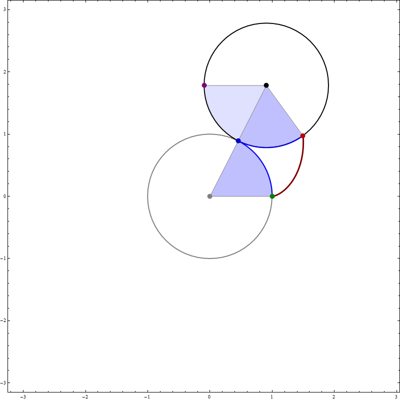
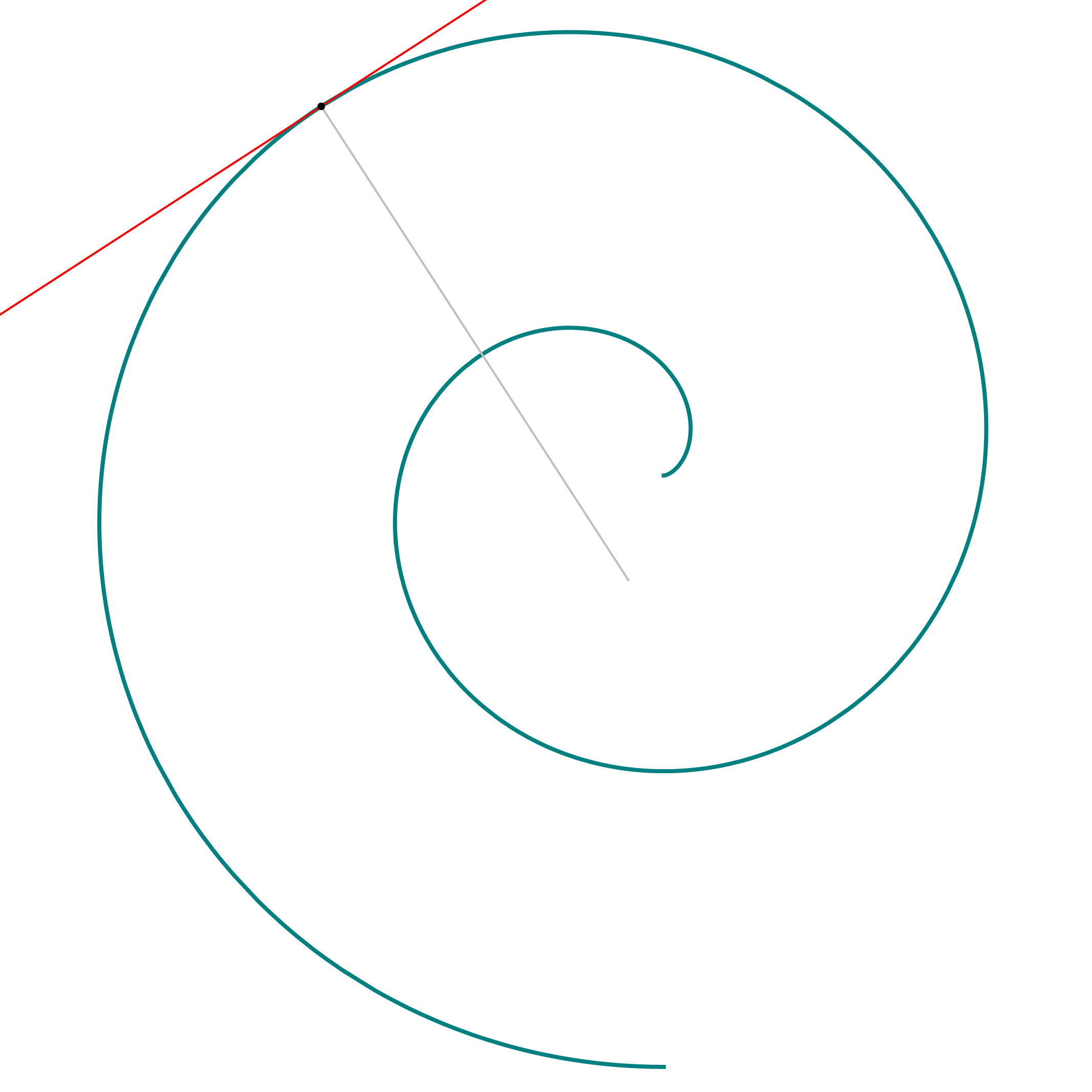
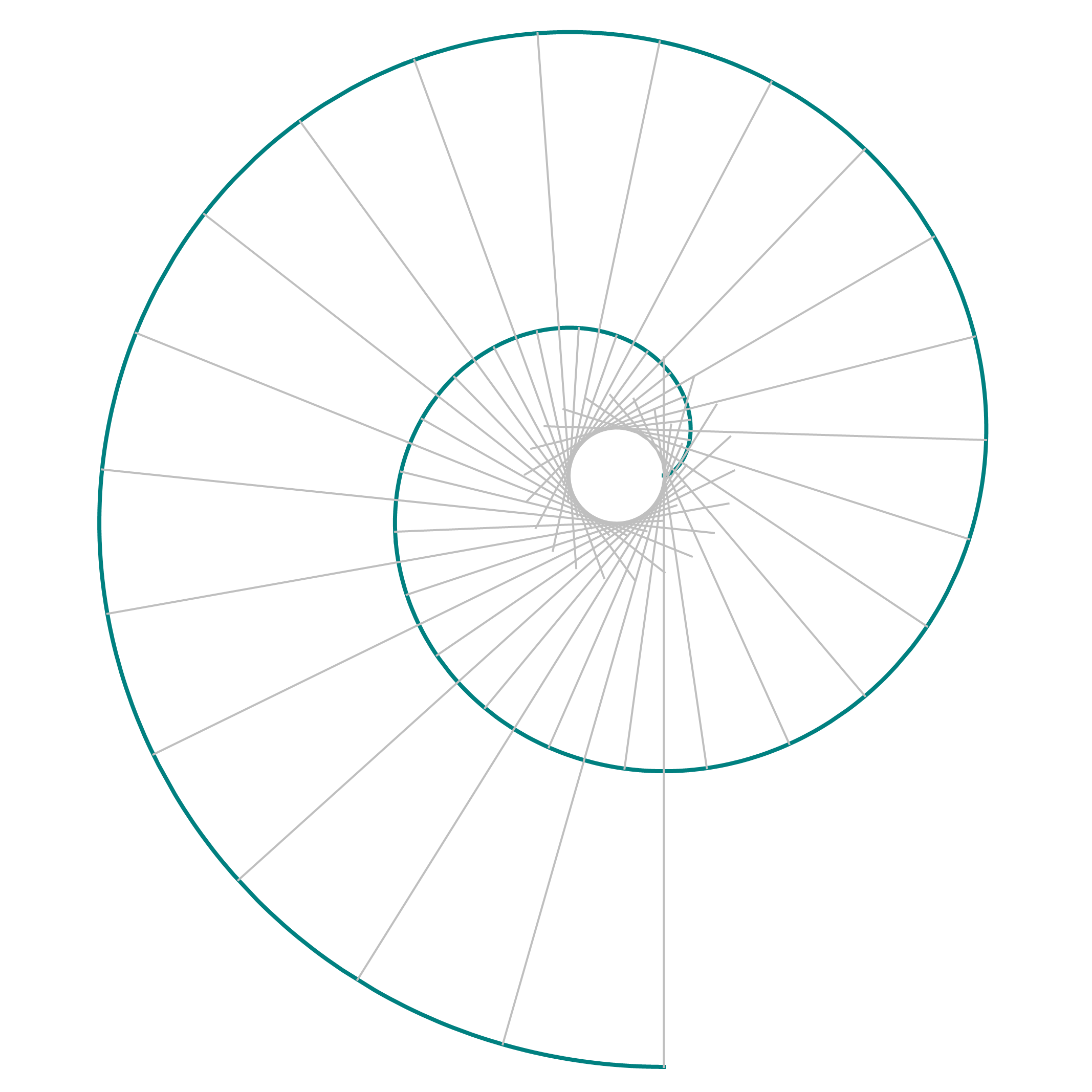
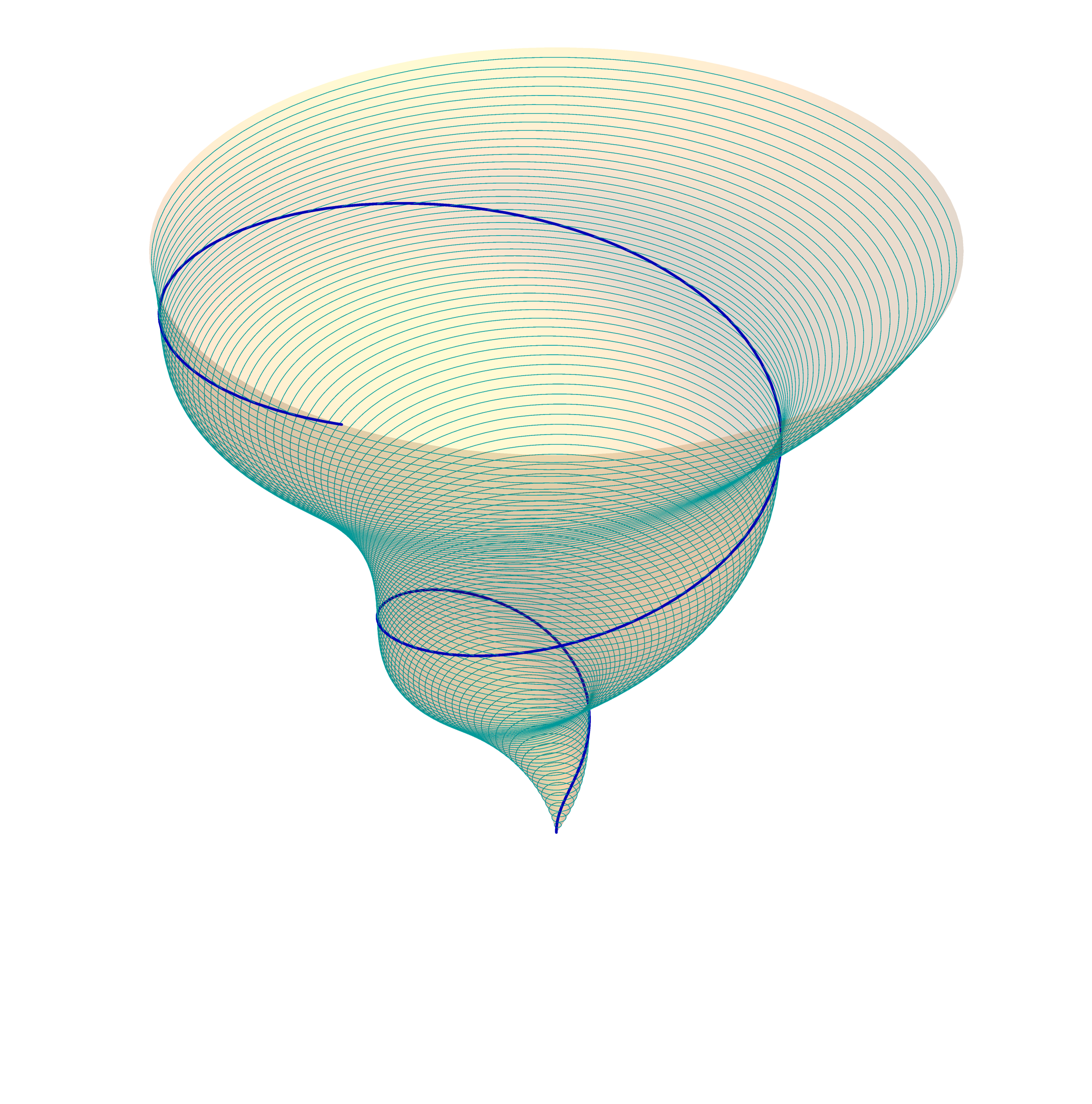
 And some artistic images inspired by this theme


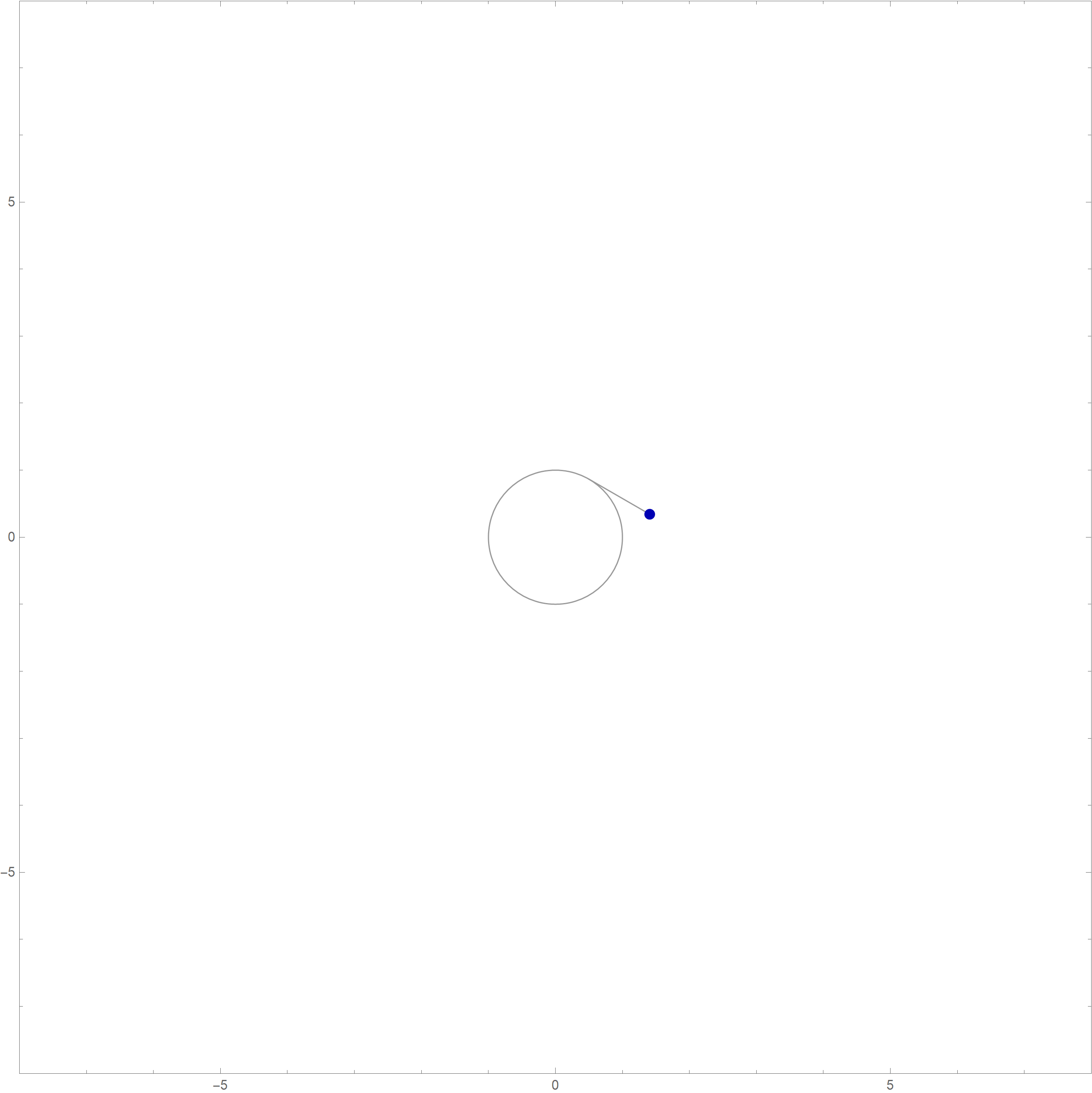
 Mathematica's command which created the complete involute of the unit circle
in the preceding image is
Mathematica's command which created the complete involute of the unit circle
in the preceding image is
 Mathematica's command for the teal circles is


 See the