- On Thursday and Friday we discussed Problem 3 on Assignment 2: explorations around Goldbach's conjecture. The summaries of the classroom presentations are in the files located in our shared OneDrive directory \Math307\2026\.
-
In Problem 3 Part (b) we explore all distinct Goldbach partitions of even integers greater than $4$. In fact, we are interested only in the count of distinct Goldbach partitions for each even integer; call this count the Goldbach length of an even number. For example, \begin{align*} 32 &= 3 +29 = 13+19, \\ 34 &= 3 + 31 = 5 + 29 = 11 + 23 = 17 + 17, \\ 36 & = 5+31 = 7+29 = 13+23 = 17 + 19. \end{align*} Hence, \(32\) has two Goldbach partitions, \(34\) has four Goldbach partitions, \(36\) has four Goldbach partitions.
The even number less than \(100\) with the largest number of Goldbach partitions is \(90\): \begin{align*} 90 & =7 + 83 = 11 + 79 = 17+ 73 \\ & = 19 + 71 = 23+ 67 = 29 + 61 \\ & = 31 + 59 = 37 + 53 = 43 + 47. \end{align*}
The following command will give all the Goldbach partitions for the even number en
Clear[AllGPs, en];
AllGPs[en_Integer?EvenQ] :=
 Select[Prime[#]&/@ Range[PrimePi[en/2]], PrimeQ[en - #] &]
In the command above, the condition Integer?EvenQ on the variable will tell Mathematica not to do any work if it is given a number which is not an even integer. The Mathematica output for AllGPs[33] is just repeated input AllGPs[33]. The same for AllGPs[Pi].
To get a list of pairs of even numbers and their Goldbach lengths, execute
{#, Length[AllGPs[#]]} & /@ Range[6, 104, 2]The output is
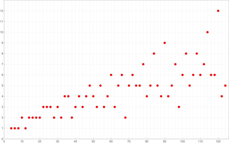
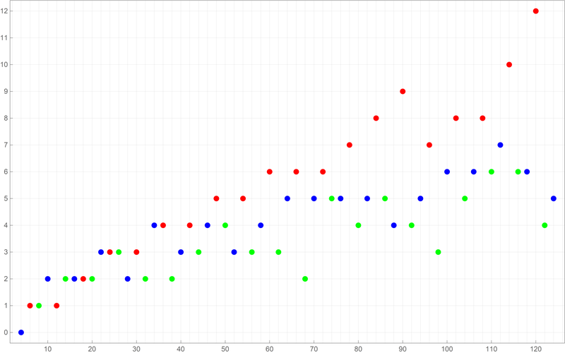
{{6, 1}, {8, 1}, {10, 2}, {12, 1}, {14, 2}, {16, 2}, {18, 2},
  {20, 2}, {22, 3}, {24, 3}, {26, 3}, {28, 2}, {30, 3}, {32, 2},
  {34, 4}, {36, 4}, {38, 2}, {40, 3}, {42, 4}, {44, 3}, {46, 4},
  {48, 5}, {50, 4}, {52, 3}, {54, 5}, {56, 3}, {58, 4}, {60, 6},
  {62, 3}, {64, 5}, {66, 6}, {68, 2}, {70, 5}, {72, 6}, {74, 5},
  {76, 5}, {78, 7}, {80, 4}, {82, 5}, {84, 8}, {86, 5}, {88, 4},
  {90, 9}, {92, 4}, {94, 5}, {96, 7}, {98, 3}, {100, 6}, {102, 8},
 {104, 5}, {106, 6}, {108, 8}, {110, 6}, {112, 7}, {114, 10},
 {116, 6}, {118, 6}, {120, 12}, {122, 4}, {124, 5}}
Below is a plot of the above first sixty values of the Goldbach lengths. Reproduce the image below.
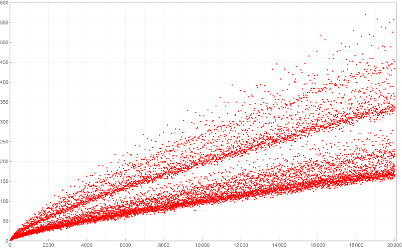
Below is a plot of the first ten thousand values of the Goldbach lengths. Reproduce the image below.
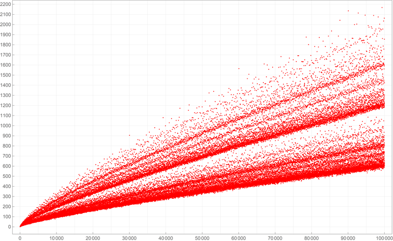
Below is a plot of the first fifty thousand values of the Goldbach lengths. Reproduce the image below.
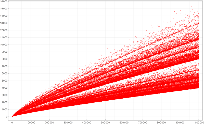
Below is a plot of the first five hundred thousand values of the Goldbach lengths. I wanted to create my own version of the picture from Wikipedia. If you can, reproduce the image below.
-
In Problem 2 Part (b-4) we explore:
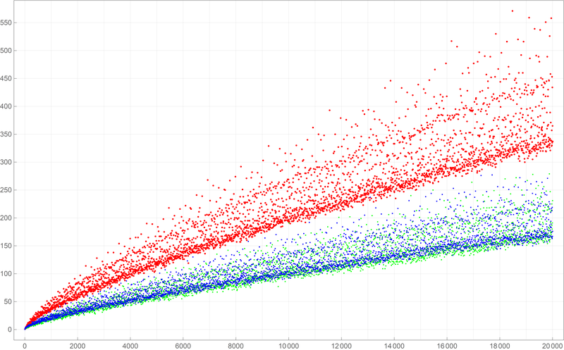
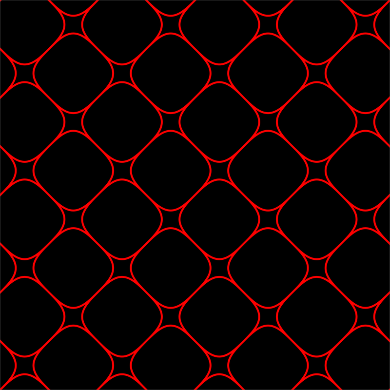
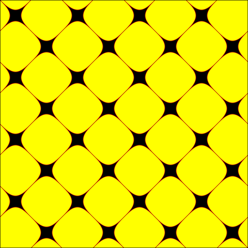
- the Goldbach lengths of the even numbers which are divisible by $6$ (colored red in the plots below)
- the Goldbach lengths of the even numbers which leave remainder $2$ when divided by $6$ (colored green in the plots below)
- the Goldbach lengths of the even numbers which leave remainder $4$ when divided by $6$ (colored blue in the plots below)
 Below is a colored plot of the first ten thousand values of the Goldbach lengths. Reproduce one of the two images below.
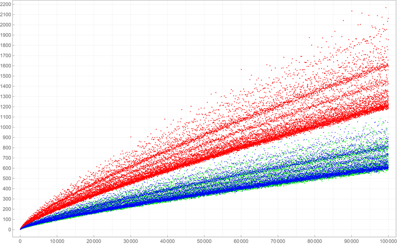
 Below is a colored plot of the first fifty thousand values of the Goldbach lengths. Reproduce one of the two images: one above, one below.
 Below is a colored plot of the first five hundred thousand values of the Goldbach lengths. I wanted to create a colored version of the picture from Wikipedia. If you can, reproduce the image below.
-
Clearly the pictures above indicate that the even numbers which are divisible by $6$ have more Goldbach partitions than those even numbers which are not divisible by $6.$ Also, the pictures indicate that there is no significant difference between the number of Goldbach partitions of the even numbers which leave remainder $2$ when divided by $6$ and the even numbers which leave remainder $4$ when divided by $6$. How to provide statistical evidence for these claims?
-
In Problem 3 Part (c) we explore the conjecture that for every odd integer $n$ greater than $3$ there exist a nonnegative integer $a$ and a prime $p$ such that
\[
n = 2 a^2 + p.
\]
To explore this conjecture one can use the idea which was used in Problem 2 Part (a). To get an idea how to organize While[] command to do a search, let us test the odd integer $57$. We start from $a=0$.
- $a=0$. Is $57- 2*0^2 = 57$ a prime number. No it is not.
- $a=1$. Is $57- 2*1^2 = 55$ a prime number. No it is not.
- $a=2$. Is $57- 2*2^2 = 49$ a prime number. No it is not.
- $a=3$. Is $57- 2*3^2 = 39$ a prime number. No it is not.
- $a=4$. Is $57- 2*4^2 = 25$ a prime number. No it is not.
- $a=5$. Is $57- 2*5^2 = 7$ a prime number. Yes it is.
- Stop. The conjecture is true for $57$ since $57 = 2*5^2 + 7$.
- Since all prime numbers are positive, we must have \[ 2 a^2 \lt 57. \] Thus we need to test only nonnegative integers $a$ such that \[ 0 \leq a \leq \left\lfloor \sqrt{\frac{57}{2}} \right\rfloor. \] Here \(\lfloor x \rfloor\) denotes the floor of a real number \(x\). In Mathematica it is Floor[].
- If we find an odd integer $n$ greater than $3$ for which all nonnegative integers $a$ such that \[ 0 \leq a \leq \left\lfloor \sqrt{\frac{n}{2}} \right\rfloor \] result with a composite positive integer \[ n - 2 a^2, \] then the stated conjecture is not true.
- Based on the analysis in the preceding item, one should organize a search, as in Problem 2 Part (a), and test several tens of thousands of odd integers greater than $3$.
-
On Thursday and Friday we explored an amazing function \[ \forall\mkern 1mu x \in \mathbb{R} \qquad x \mapsto \frac{\sin (x)+\tanh (x)}{1 + \sin (x) \tanh (x)}. \]
In the Mathematica code below, I will consistently write this function as a pure function:
(Sin[#] + Tanh[#])/(1 + Sin[#] Tanh[#]) &
I find this preferable to assigning it a name, since it keeps us constantly aware of the function's spirit: Sin[#]& and Tanh[#]&.
-
Before preceding with the explorations of the given function, let us review what we know about its components
Plot[Sin[#] &[x], {x, -2 Pi, 2 Pi}, PlotStyle -> {Thickness[0.005]},
 Epilog -> {{PointSize[0.0125], RGBColor[0.7 {0, 0, 1}],
    Point[{#, Sin[#]}] & /@
     Range[-4 Pi + Pi/2, 4 Pi, 2 Pi]}, {PointSize[0.0125],
    RGBColor[0.7 {0, 1, 0}],
    Point[{#, Sin[#]}] & /@ Range[-4 Pi + (3 Pi)/2, 4 Pi, 2 Pi]}},
 Ticks -> {Range[-4 Pi, 4 Pi, Pi/2], Automatic}]
Plot[Tanh[#] &[x], {x, -8, 8}, PlotStyle -> {Thickness[0.005]},
 Epilog -> {{Thickness[0.003], RGBColor[0.7 {0, 0, 1}],
    Line[{{{-10, 1}, {10, 1}}}]}, {Thickness[0.003],
    RGBColor[0.7 {0, 1, 0}], Line[{{{-10, -1}, {10, -1}}}]}},
 Ticks -> {Range[-10, 10, 1], Automatic}]
We see that Tanh[#]& is an odd sigmoid function with the horizontal asymptotes at \(y=1\) and \(y=-1\) and that Tanh[#]& approaches the asymptotes very rapidly. In fact \begin{align*} \tanh(20) &\approx 0.99999999999999999150329148941682204543855819119099\\ \tanh(50) &\approx 0.99999999999999999999999999999999999999999992559848 \end{align*}
-
A basic Plot[...] results in
Plot[(Sin[#] + Tanh[#])/(1 + Sin[#] Tanh[#])&[x], {x, -9, 9}, PlotStyle -> {Thickness[0.005]}]
The graph indicates that the function is odd: \[ \forall\mkern 1mu x \in \mathbb{R} \quad \frac{\sin (-x)+\tanh (-x)}{1 + \sin (-x) \tanh (-x)} = \frac{-\sin (x)-\tanh (x)}{1 + \sin (x) \tanh (x)} = - \frac{\sin (x)+\tanh (x)}{1 + \sin (x) \tanh (x)} \] Thus for all the features we can focus on the positive real numbers.
-
Natural questions arise: Is this function defined for all real numbers? What is the exact range of this function?
-
To understand this function we have to use our knowledge of its components Sin[#]& and Tanh[#]&.
We know that
Sin[#] & /@ Range[-10 Pi + Pi/2, 10 Pi, 2 Pi]
will result in all 1s. While
Sin[#] & /@ Range[-10 Pi + 3 Pi/2, 10 Pi, 2 Pi]
will result in all -1s.
Therefore it is interesting to evaluate our given function at those values. And we can do that "on paper". For every integer \(k\) we have \[ \frac{\sin \bigl(\tfrac{\pi}{2}+2 k \pi\bigr)+\tanh(\tfrac{\pi}{2}+2 k \pi\bigr)}{1 + \sin(\tfrac{\pi}{2}+2 k \pi\bigr) \tanh(\tfrac{\pi}{2}+2 k \pi\bigr)} = \frac{1+\tanh(\tfrac{\pi}{2}+2 k \pi\bigr)}{1 + 1 \tanh(\tfrac{\pi}{2}+2 k \pi\bigr)} = \Large 1 \] and \[ \frac{\sin \bigl(\tfrac{3\pi}{2}+2 k \pi\bigr)+\tanh(\tfrac{3\pi}{2}+2 k \pi\bigr)}{1 + \sin(\tfrac{3\pi}{2}+2 k \pi\bigr) \tanh(\tfrac{3\pi}{2}+2 k \pi\bigr)} = \frac{-1+\tanh(\tfrac{\pi}{2}+2 k \pi\bigr)}{1 + (-1) \tanh(\tfrac{\pi}{2}+2 k \pi\bigr)} = - \Large 1 \]
There is a warning in the denominator of the last expression \[ 1 + (-1) \tanh(\tfrac{\pi}{2}+2 k \pi\bigr) = 1 - \tanh(\tfrac{\pi}{2}+2 k \pi\bigr). \] We have seen earlier that \(\tanh(50)\) is very close to \(1\). So when the positive integer \(k\) is large, \(\tanh(\tfrac{\pi}{2}+2 k \pi\bigr)\) is very close to \(0\). It can be so close to \(0\) that Mathematica can mistakenly take it to be \(0\). We need to be aware of this in out calculations.
-
Let us implement what we calculated in the preceding item on a graph of the given function.
Plot[(Sin[#] + Tanh[#])/(1 + Sin[#] Tanh[#]) &[x], {x, 0, 30},
 PlotStyle -> {Thickness[0.005]},
 Epilog -> {{PointSize[0.0125], RGBColor[0.7 {0, 0, 1}],
    Point[{#, (Sin[#] + Tanh[#])/(1 + Sin[#] Tanh[#])}] & /@
     Range[-4 Pi + Pi/2, 40 Pi, 2 Pi]}, {PointSize[0.0125],
    RGBColor[0.7 {0, 1, 0}],
    Point[{#,
        FullSimplify[(Sin[#] + Tanh[#])/(1 + Sin[#] Tanh[#])]}] & /@
     Range[-4 Pi + (3 Pi)/2, 40 Pi, 2 Pi]}},
 PlotRange -> {{0, 30}, {-1.1, 1.1}},
 Ticks -> {Range[-4 Pi, 40 Pi, Pi/2], Automatic}]
This graph clearly indicates that something suspicious is going on with this graph. What is happening near the \(x\)-values \(\dfrac{3\pi}{2}+2 k \pi\) for nonnegative values of the integer \(k\)?
This needs additional explorations.
-
I decided that it will be a good idea to zoom in near the \(x\)-values \[ \dfrac{3\pi}{2}, \quad \dfrac{3\pi}{2}+2 \pi, \quad \dfrac{3\pi}{2}+4 \pi, \quad \dfrac{3\pi}{2}+6 \pi, \ldots \]
To automate this process, I introduced the variable nn for the number of \(2\pi\) that I am adding and the variable dx for the range of the variable \(x\) that I am allowing. So, I graph the given function on the interval
{x, 2 nn Pi + (3 Pi)/2 - dx, 2 nn Pi + (3 Pi)/2 + dx}I choose the following PlotRange->
PlotRange ->
{{2 nn Pi + (3 Pi)/2 - dx,  2 nn Pi + (3 Pi)/2 + dx}, {-1.1, 1.1}}
In the command below I use Module[] to make the variables nn and dx local.
Module[{nn, dx}, nn = 1; dx = (3/2) 10^(-4);
 Plot[(Sin[#] + Tanh[#])/(1 + Sin[#] Tanh[#]) &[x] , {x,
   2 nn Pi + (3 Pi)/2 - dx, 2 nn Pi + (3 Pi)/2 + dx},
  PlotPoints -> 1500, PlotStyle -> {Thickness[0.005]},
  PlotRange -> {{2 nn Pi + (3 Pi)/2 - dx,
     2 nn Pi + (3 Pi)/2 + dx}, {-1.1, 1.1}},
  Epilog -> {{Text[
      2 nn Pi + (3 Pi)/2, {2 nn Pi + (3 Pi)/2, 0.15}]}, {PointSize[
      0.01], RGBColor[0, 0.6, 0],
     Point[{#, -1}] & /@
      Range[2 (nn - 1) Pi + (3 Pi)/2, 2 (nn + 1) Pi + (3 Pi)/2,
       2 Pi]}}, Axes -> True,
  Ticks -> {{#, N[#]} & /@
     Range[2 nn Pi + (3 Pi)/2 - dx, 2 nn Pi + (3 Pi)/2 + dx, dx/4],
    Automatic}, ImageSize -> 800]]
Module[{nn, dx}, nn = 2; dx = (3/2) 10^(-6);
 Plot[(Sin[#] + Tanh[#])/(1 + Sin[#] Tanh[#]) &[x] ,
  {x, 2 nn Pi + (3 Pi)/2 - dx, 2 nn Pi + (3 Pi)/2 + dx},
  PlotPoints -> 1500, PlotStyle -> {Thickness[0.005]},
  PlotRange -> {{2 nn Pi + (3 Pi)/2 - dx,
     2 nn Pi + (3 Pi)/2 + dx}, {-1.1, 1.1}},
  Epilog -> {{Text[
      2 nn Pi + (3 Pi)/2, {2 nn Pi + (3 Pi)/2, 0.15}]}, {PointSize[
      0.01], RGBColor[0, 0.6, 0],
     Point[{#, -1}] & /@
      Range[2 (nn - 1) Pi + (3 Pi)/2, 2 (nn + 1) Pi + (3 Pi)/2,
       2 Pi]}}, Axes -> True,
  Ticks -> {{#, N[#]} & /@
     Range[2 nn Pi + (3 Pi)/2 - dx, 2 nn Pi + (3 Pi)/2 + dx, dx/4],
    Automatic}, ImageSize -> 800]]
Module[{nn, dx}, nn = 3; dx = (3/2) 10^(-8);
 Plot[(Sin[#] + Tanh[#])/(1 + Sin[#] Tanh[#])&[x],
 {x, 2 nn Pi + (3 Pi)/2 - dx, 2 nn Pi + (3 Pi)/2 + dx},
  PlotPoints -> 1500, PlotStyle -> {Thickness[0.005]},
  PlotRange -> {{2 nn Pi + (3 Pi)/2 - dx,
     2 nn Pi + (3 Pi)/2 + dx}, {-1.1, 1.1}},
  Epilog -> {
  {Text[2 nn Pi + (3 Pi)/2, {2 nn Pi + (3 Pi)/2, 0.15}]},
  {PointSize[0.01], RGBColor[0, 0.6, 0],
     Point[{#, -1}]&/@
 Range[2 (nn - 1) Pi + (3 Pi)/2, 2 (nn + 1) Pi + (3 Pi)/2, 2 Pi]}},
  Axes -> True, Ticks -> {{#, N[#]}&/@
     Range[2 nn Pi + (3 Pi)/2 - dx, 2 nn Pi + (3 Pi)/2 + dx, dx/4],
    Automatic}, ImageSize -> 800]]
But, unfortunately, this strategy does not work for nn = 3. The last graph above is not very informative. Even worse, when we zoom in to dx = (3/2) 10^(-9), Mathematica reports errors. I illustrate the errors just by numerical calculations below.
Module[{nn, dx}, nn = 3; dx = (3/2)*10^-(9);
 N[ (Sin[#] + Tanh[#])/(1 + Sin[#] Tanh[#])] & /@
  Range[2 nn Pi + (3 Pi)/2 - dx, 2 nn Pi + (3 Pi)/2 + dx, dx/4]]
Resulting in
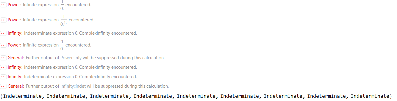
But, by carefully considering our calculations above we understand the source for these errors. Mathematica thinks that it encounters zero in the denominator. It is possible that we overcome this problem if we increase the precision with which Mathematica does the calculations. We do that in the next item.
-
To overcome the calculational problem at the end of the preceding item, we use SetPrecision[].
Module[{nn, dx}, nn = 3; dx = (3/2)*10^-(9);
 N[SetPrecision[(Sin[#] + Tanh[#])/(1 + Sin[#] Tanh[#]), 100]] & /@
  Range[2 nn Pi + (3 Pi)/2 - dx, 2 nn Pi + (3 Pi)/2 + dx, dx/4]]
Resulting in

These numbers are not extreme. The extremely small numbers are in the denominator of the given function.
I was not able to use SetPrecision[] in Plot[]. A solution that I found is in the next item.
-
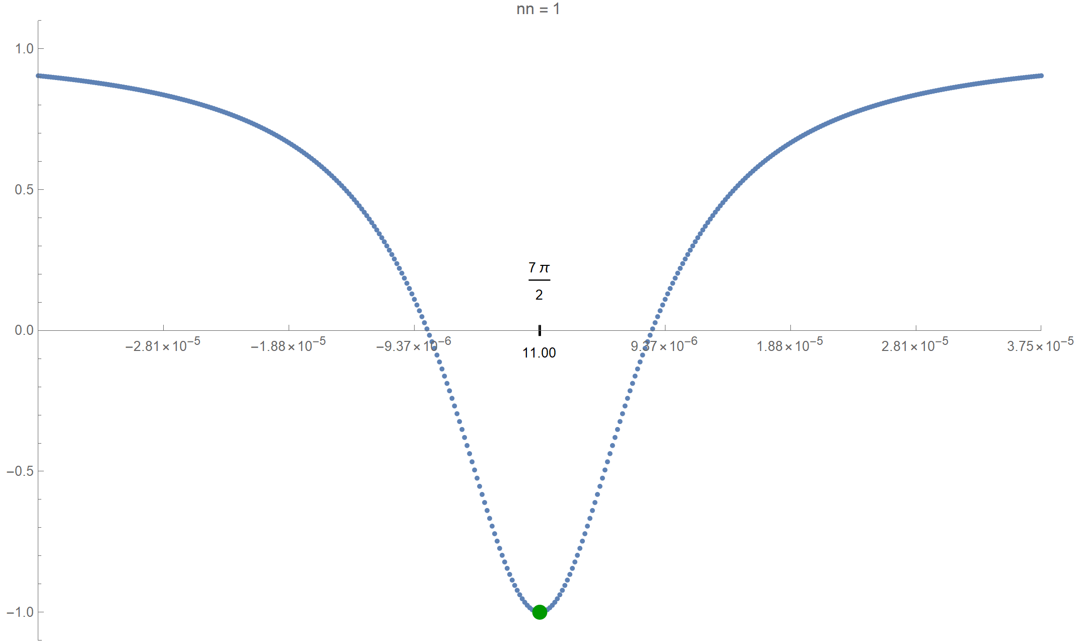
I decided to replace Plot[] with just plotting points on the graph of the given function in Graphics[]. Also, instead graphing the given function near \[ \dfrac{3\pi}{2}, \quad \dfrac{3\pi}{2}+2 \pi, \quad \dfrac{3\pi}{2}+4 \pi, \quad \dfrac{3\pi}{2}+6 \pi, \quad \ldots, \quad \dfrac{3\pi}{2}+2 k \pi \] for large positive integers \(k\), I shift the function to the left, and plot the shifted function near \(0\); the shifted function being \[ \forall\mkern 1mu x \in (-1, 1) \qquad x \mapsto \frac{\sin\bigl(\delta x + \tfrac{3 \pi}{2} + 2 k \pi\bigr) + \tanh\bigl(\delta x + \tfrac{3 \pi}{2} + 2 k \pi\bigr)} {1 + \sin\bigl(\delta x + \tfrac{3 \pi}{2} + 2 k \pi\bigr) \tanh\bigl(\delta x + \tfrac{3 \pi}{2} + 2 k \pi\bigr)}. \] Here I use \(\delta \gt 0\) instead of dx and \(k\) instead of nn for a nonnegative integer.
Module[{dx, pws, nn}, nn = 12;
 (* dx below is the small range of x, how small is given with the \
powers 10^(-1) from the list below  *)
 pws = {4, 7, 9, 12, 15, 17, 20, 23, 26, 28, 31, 34, 37, 39, 42, 45,
   47, 50, 53, 56, 58, 61, 64, 67, 69, 72, 75, 77, 80, 83, 86, 88, 91,
    94, 96, 99, 102, 105, 107, 110, 113, 116, 118, 121, 124, 126, 129,
    132, 135, 137};
 dx = 3/2*10^-pws[[nn]];
 Graphics[{
   (* Below are 201 points on the graph near the value 2nn Pi+(3 Pi)/
   2 *)

   {PointSize[0.005], RGBColor[0.37, 0.51, 0.71],
    Point[{#,
        SetPrecision[(
         Sin[dx # + (3 Pi)/2] + Tanh[dx # + 2 nn Pi + (3 Pi)/2])/(
         1 + Sin[dx # + (3 Pi)/2] Tanh[dx # + 2 nn Pi + (3 Pi)/2]),
         300]}] & /@ Range[-1, 1, (1/2)*10^(-2)]},
   (* Which point is considered is shown below,
   exact and approximate *)
    {Text[2 nn Pi + (3 Pi)/2, {0, 0.175}],
    Text[N[2 nn Pi + (3 Pi)/2, 4], {0, -0.08}]},

   (* below is the tickmark at the minimum shown *)
   {Thickness[0.003], Line[{{0, -0.015}, {0, 0.015}}]},
   (* the dark green minimum point of the function *)
   {PointSize[0.015], RGBColor[0.6 {0, 1, 0}], Point[{0, -1}]}
   },
  Axes -> True, AspectRatio -> 1/GoldenRatio,
  PlotRangePadding -> None, Frame -> False,
  Ticks -> {If[Abs[#] > 0.1, {#, (dx/3) #}, {#, ""}] & /@
     Range[-1, 1, 0.25], Automatic},
  PlotRange -> {{-1, 1}, {-1.1, 1.1}}, AxesOrigin -> {-1, 0},
  PlotLabel ->
   TableForm[{"nn =", nn}, TableDirections -> Row,
    TableSpacing -> 0.3], ImageSize -> 600]]
Click on the image below to see the zoomed graphs.
-
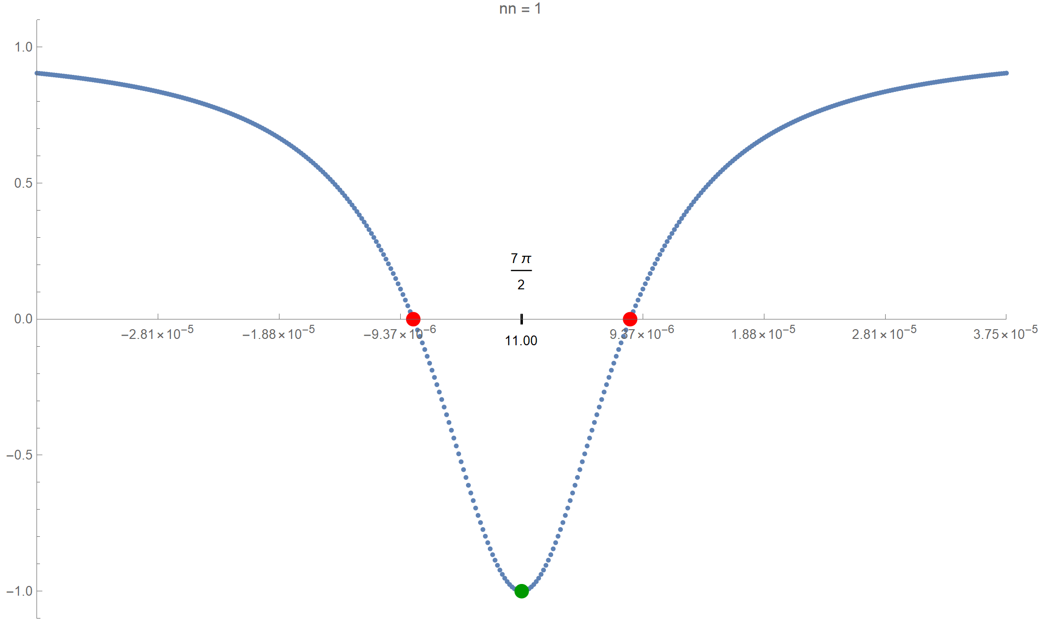
Finally, I want to calculate the \(x\)-intercepts near each minimum.
Module[{dx, pws, zxl, zxr, nn}, nn = 16;
 pws = {4, 7, 9, 12, 15, 17, 20, 23, 26, 28, 31, 34, 37, 39, 42, 45,
   47, 50, 53, 56, 58, 61, 64, 67, 69, 72, 75, 77, 80, 83, 86, 88, 91,
    94, 96, 99, 102, 105, 107, 110, 113, 116, 118, 121, 124, 126, 129,
    132, 135, 137};
 dx = 3/2*10^-pws[[nn]];
(* below we use FindRoot with Brent method to calculate the
x-intercepts first the left one then the right one *)
zxl = (x /. FindRoot[
     ff[x] == 0, {x, (3 Pi)/2 + 2 nn Pi - 1/1000, (3 Pi)/2 + 2 nn Pi},
      MaxIterations -> 2000, WorkingPrecision -> 200,
     Method -> "Brent"]);
 zxr = (x /.FindRoot[
     ff[x] == 0, {x, (3 Pi)/2 + 2 nn Pi, (3 Pi)/2 + 2 nn Pi + 1/1000},
      MaxIterations -> 2000, WorkingPrecision -> 200,
     Method -> "Brent"]);
 Graphics[{
   {PointSize[0.005], RGBColor[0.37, 0.51, 0.71],
    Point[{#,
        SetPrecision[(
         Sin[dx # + (3 Pi)/2] + Tanh[dx # + 2 nn Pi + (3 Pi)/2])/(
         1 + Sin[dx # + (3 Pi)/2] Tanh[dx # + 2 nn Pi + (3 Pi)/2]),
         300]}] & /@ Range[-1, 1, (1/2) 10^-2]},
   {PointSize[0.015], RGBColor[1, 0, 0],
    Point[{(zxl - ((3 Pi)/2 + 2 nn Pi))/dx , 0}],
    Point[{(zxr - ((3 Pi)/2 + 2 nn Pi))/dx , 0}]},
     {Text[2 nn Pi + (3 Pi)/2, {0, 0.175}],
    Text[N[2 nn Pi + (3 Pi)/2, 4], {0, -0.08}]}, {Thickness[0.003],
    Line[{{0, -0.015}, {0, 0.015}}]}, {PointSize[0.015],
    RGBColor[0, 0.6, 0], Point[{0, -1}]}
   },
  Axes -> True, AspectRatio -> 1/GoldenRatio,
  PlotRangePadding -> None, Frame -> False,
  Ticks -> {If[
       Abs[#] > 0.1, {#, ScientificForm[(dx/4) #, {3, 2}]}, {#,
        ""}] & /@ Range[-1, 1, 0.25], Automatic},
  PlotRange -> {{-1, 1}, {-1.1, 1.1}}, AxesOrigin -> {-1, 0},
  PlotLabel ->
   TableForm[{"nn =", nn}, TableDirections -> Row,
    TableSpacing -> 0.3], ImageSize -> 800]]
Click on the image below to see the zoomed graphs with the \(x\)-intercepts.
- I need to write here about the arc length and the chord length of a circle. It is a beautiful story of the inevitability and omnipresence of bijections.
- On Friday in class I showed how to make tori from the regular \(n\)-gons we introduced earlier. An interesting next goal is to create a twisted \(n\)-gon torus, in particular a twisted triangular torus (called a toroid).
- Below I present two animations which show two ways to construct the one-third-twisted triangular toroid.
-
In this item, the one-third-twisted triangular toroid is constructed by a rotating equilateral triangle. The triangle is rotated by the full circle, that is the angle $2\pi$.
Place the cursor over the image to start the animation.
The code that is used for the above picture (not the animation) is below:
Show[ParametricPlot3D[
  3 {Cos[s], Sin[s], 0} +
   NgonCos[t, 3] (Cos[s/3] {Cos[s], Sin[s], 0} + Sin[s/3] {0, 0, 1}) +
    NgonSin[t,3] (-Sin[s/3] {Cos[s], Sin[s], 0} + Cos[s/3] {0, 0, 1}), {t, 0,
   3}, {s, 0, 2 Pi}, PlotPoints -> {51, 201},
  PlotStyle -> {Opacity[0.9]}, Mesh -> False, Exclusions -> None,
  PlotRange -> {{-4, 4}, {-4, 4}, {-1.1, 1.1}}],
 ParametricPlot3D[
  3 {Cos[s], Sin[s], 0} +
   NgonCos[0, 3] (Cos[s/3] {Cos[s], Sin[s], 0} + Sin[s/3] {0, 0, 1}) +
    NgonSin[0,
     3] (-Sin[s/3] {Cos[s], Sin[s], 0} + Cos[s/3] {0, 0, 1}), {s, 0,
   2 Pi}, PlotPoints -> {201},
  PlotStyle -> {RGBColor[0, 0, 0.75], Thickness[0.006]},
  Exclusions -> None],
 ParametricPlot3D[
  3 {Cos[s], Sin[s], 0} +
   NgonCos[1, 3] (Cos[s/3] {Cos[s], Sin[s], 0} + Sin[s/3] {0, 0, 1}) +
    NgonSin[1, 3] (-Sin[s/3] {Cos[s], Sin[s], 0} + Cos[s/3] {0, 0, 1}), {s, 0,
   2 Pi}, PlotPoints -> {201},
  PlotStyle -> {RGBColor[0.95, 0, 0], Thickness[0.006]},
  Exclusions -> None],
 ParametricPlot3D[
  3 {Cos[s], Sin[s], 0} +
   NgonCos[2, 3] (Cos[s/3] {Cos[s], Sin[s], 0} + Sin[s/3] {0, 0, 1}) +
    NgonSin[2, 3] (-Sin[s/3] {Cos[s], Sin[s], 0} + Cos[s/3] {0, 0, 1}), {s, 0,
   2 Pi}, PlotPoints -> {201},
  PlotStyle -> {RGBColor[0, 0.85, 0], Thickness[0.006]},
  Exclusions -> None], ImagePadding -> {{0, 0}, {0, 0}},
 Boxed -> True, BoxStyle -> {Opacity[0]}, Axes -> False,
 ImageSize -> 1000, PlotRange -> {{-4, 4}, {-4, 4}, {-1.1, 1.1}}]
The above code uses the functions that we defined earlier:
Clear[NgonCos, NgonSin]; NgonCos[t_, nn_] := (1 - (t - Floor[t])) Cos[(2/nn) \[Pi] Floor[t]] + (t - Floor[t]) Cos[(2/nn) \[Pi] (1 + Floor[t])]; NgonSin[t_, nn_] := (1 - (t - Floor[t])) Sin[(2/nn) \[Pi] Floor[t]] + (t - Floor[t]) Sin[(2/nn) \[Pi] (1 + Floor[t])]; -
In this item, the one-third-twisted triangular toroid is constructed by a rotating line segment. The line segment is rotated by the three full circles, that is by the angle $6\pi$.
Place the cursor over the image to start the animation.
The code that is used for the above picture (not the animation) is below:
Show[ParametricPlot3D[
  3 {Cos[s], Sin[s], 0} +
   NgonCos[t, 3] (Cos[s/3] {Cos[s], Sin[s], 0} + Sin[s/3] {0, 0, 1}) +
    NgonSin[t, 3] (-Sin[s/3] {Cos[s], Sin[s], 0} + Cos[s/3] {0, 0, 1}), {t, 0,
   1}, {s, 0, 6 Pi}, PlotPoints -> {51, 201},
  PlotStyle -> {Opacity[0.9]}, Mesh -> False, Exclusions -> None,
  PlotRange -> {{-4, 4}, {-4, 4}, {-1.1, 1.1}}],
 ParametricPlot3D[
  3 {Cos[s], Sin[s], 0} +
   NgonCos[0, 3] (Cos[s/3] {Cos[s], Sin[s], 0} + Sin[s/3] {0, 0, 1}) +
    NgonSin[0, 3] (-Sin[s/3] {Cos[s], Sin[s], 0} + Cos[s/3] {0, 0, 1}), {s, 0,
   6 Pi}, PlotPoints -> {201},
  PlotStyle -> {RGBColor[0, 0, 0.75], Thickness[0.006]},
  Exclusions -> None], ImagePadding -> {{0, 0}, {0, 0}},
 Boxed -> True, BoxStyle -> {Opacity[0]}, Axes -> False,
 ImageSize -> 1000, PlotRange -> {{-4, 4}, {-4, 4}, {-1.1, 1.1}}]
The above code uses the functions that we defined earlier:
Clear[NgonCos, NgonSin];
NgonCos[t_, nn_] := (1 - (t - Floor[t])) Cos[(2/nn) \[Pi] Floor[t]] + (t -
      Floor[t]) Cos[(2/nn) \[Pi] (1 + Floor[t])];
NgonSin[t_, nn_] := (1 - (t - Floor[t])) Sin[(2/nn) \[Pi] Floor[t]] + (t -
      Floor[t]) Sin[(2/nn) \[Pi] (1 + Floor[t])];
- It is important in life to orient oneself in the world of COLORS. To help with that, I wrote a webpage: Color Cube. And all illustrations on the Color Cube page are created in Mathematica.
- Being able to navigate the world of C O L O R S is important. To help with this, I created a page: Color Cube. All illustrations on the Color Cube page were generated using Mathematica.
-
One of the remarkable applications of trigonometric functions Cos[t] and Sin[x] is that they describe small oscillations of a stretched string. In the animation below you can see the function \[ \cos(t) \sin(x) \qquad \text{with} \qquad x \in [0,\pi] \quad \text{and} \quad t \in [0,2\pi] \] As \(t\) takes values from \(0\) to \(2\pi\), the function \(\sin(x)\) is scaled with a different number \(\cos(t)\) between \(1\) and \(-1\). In the animation below I take 241 values of \(t\) between, and including, \(0\) to \(2\pi\), create 241 images and use Mathematica to export those 241 images as an animated gif file.
Hover over the image to start the animation.
-
This is the Mathematica code used to create the above animation and export it as an animated gif file.
(* create a list of 240 images of an oscillating sine function, call \ this list SinxCost *) SinxCost = Table[Plot[Evaluate[Sin[x] Cos[t]], {x, 0, Pi}, PlotStyle -> {{Thickness[0.01], RGBColor[1, 0, 0]}}, Epilog -> { {PointSize[0.012], White, Point[#] & /@ {{0, 0}, {Pi, 0}}}, {Text["t =", {Pi/2 - 0.1, 1.26}, BaseStyle -> {FontWeight -> "Normal", FontColor -> RGBColor[1, 1, 1]}], Text[NumberForm[N[t], {3, 2}], {Pi/2, 1.26}, BaseStyle -> {FontWeight -> "Normal", FontColor -> RGBColor[1, 1, 1]}]} }, PlotRange -> {{-0.1, Pi + 0.1}, {-1.4, 1.4}}, AspectRatio -> 1/5, Frame -> True, FrameTicks -> {{{}, {}}, {Range[0, Pi, Pi/4], {}}}, Axes -> False, ImageSize -> 800, Background -> Black], {t, 0, 2 Pi, 2 Pi/240.}]; (* decide which duration you want for each frame, here 0.1 and create \ a table of these durations, call it dds *) dds = 0.1 & /@ Range[Length[SinxCost]]; (* Set the directory where you want the movie to be exported. *) SetDirectory["C:\\Dropbox\\Work\\myweb\\Courses\\Math_pages\\Math_307\ \\Pictures"] (* Export the list of 240 images as an animated gif file *) Export["SinxCostAni.gif", SinxCost, "AnimationRepetitions" -> Infinity, "ImageSize" -> 800, "DisplayDurations" -> dds] (* Export the first image as a gif file *) Export["SinxCostS1.gif", SinxCost[[1]], "ImageSize" -> 800] -
Since we worked so much with the cosine and sine function, I started playing with the graph of the sine function. I moved it around, placed it climbing along the \(y\)-axis. Then, I decided to animate each of the graphs and this turns into art.
Hover over the image to start the animation.
Hover over the image to start the animation.
Hover over the image to start the animation.
- Assignment 1 has been posted in our shared OneDrive directory \Math307\Assignments.
-
To appreciate the Beauty of Trigonometry, it is essential to understand the key feature of the trigonometric functions Cos[t] and Sin[t]:
-
The trigonometric functions Cos[t] and Sin[t] provide a parametrization of the unit circle. But that is just the beginning—most importantly, a deep understanding of the sphere and torus is impossible without Cos[t] and Sin[t].
-
-
The animation below is my attempt to illustrate how the parametrization of the unit circle works.
-
The main components of the animation are as follows:
- The black circle is the unit circle.
- The values of t $\in [0,2\pi]$ are represented by orange lengths. In each scene there are three orange lengths: the horizontal length, the vertical length and the arc length on the unit circle.
- The values of Cos[t] are green horizontal line segments.
- The values of Sin[t] are blue vertical line segments.
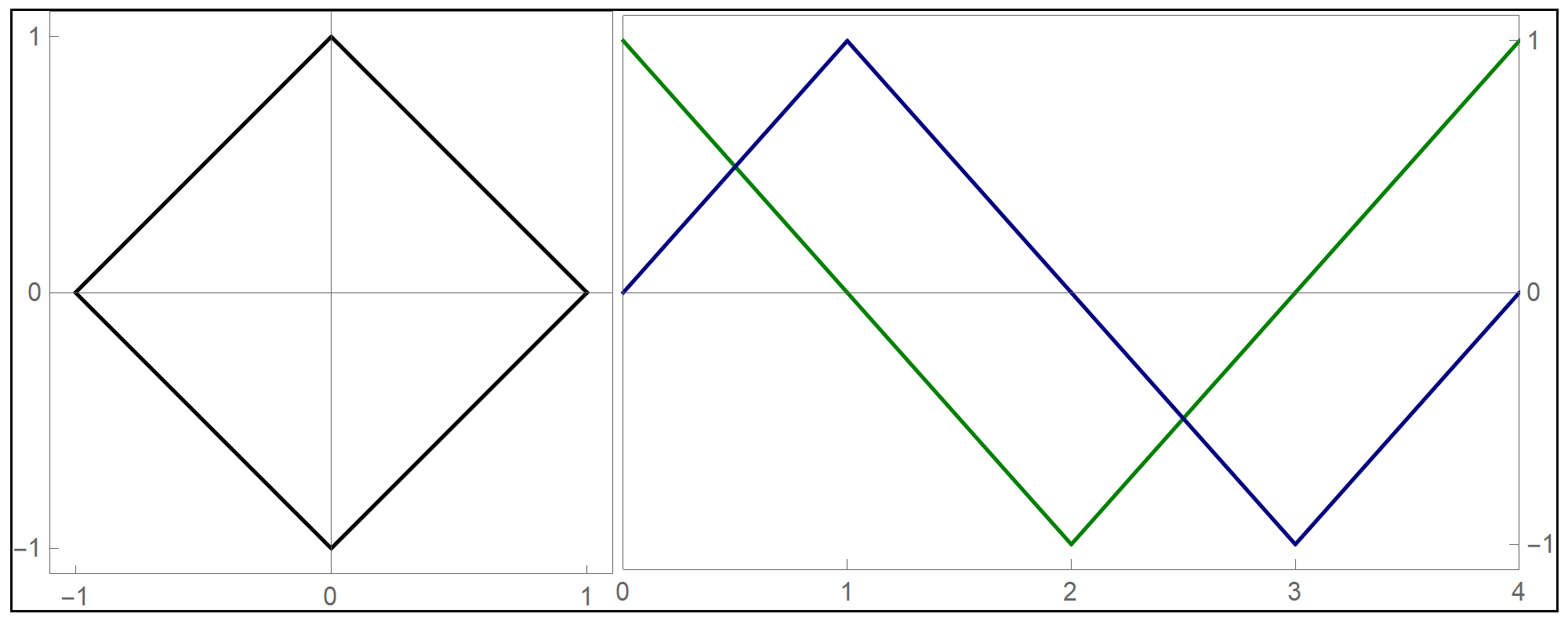
- The principle above is the general principle of parametric equations of curves in the plane. Given two functions (one green and one blue) of the same independent variable t, if these functions define the coordinates of a moving point, then as the independent variable t varies, the point traces a curve in the plane.
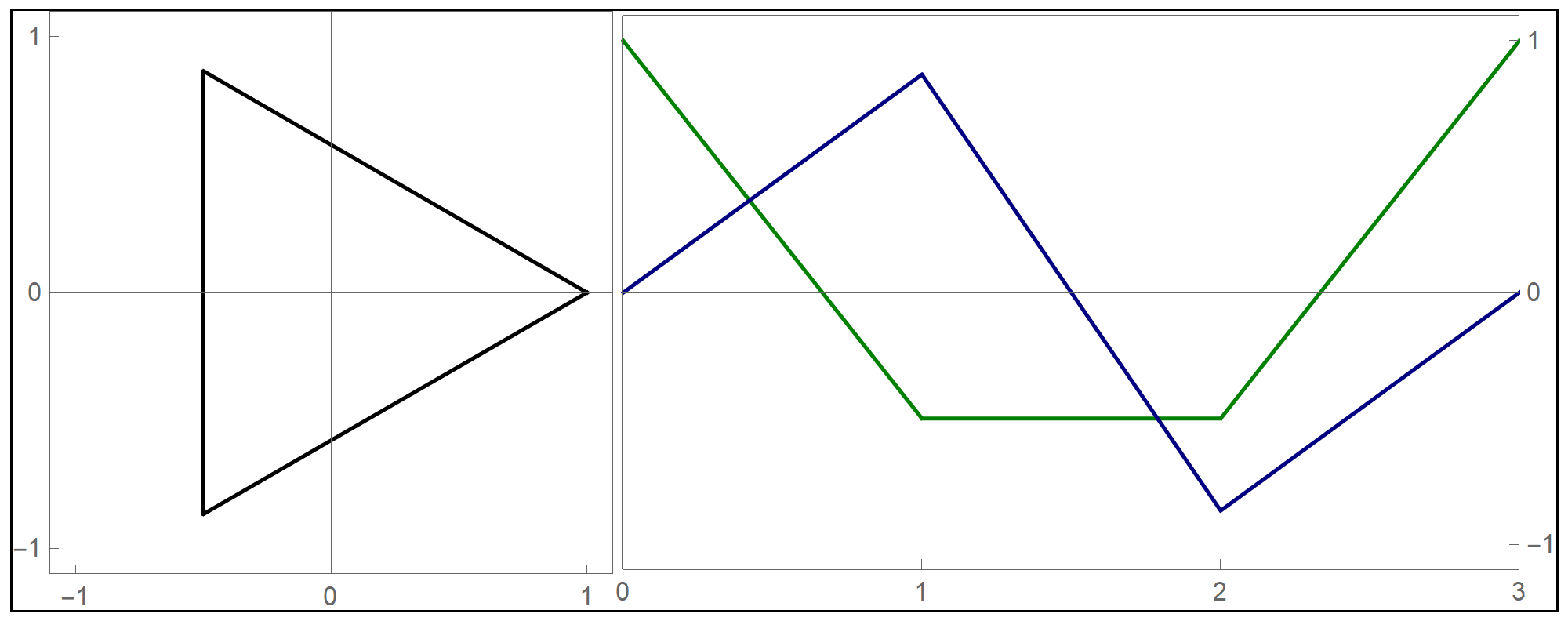
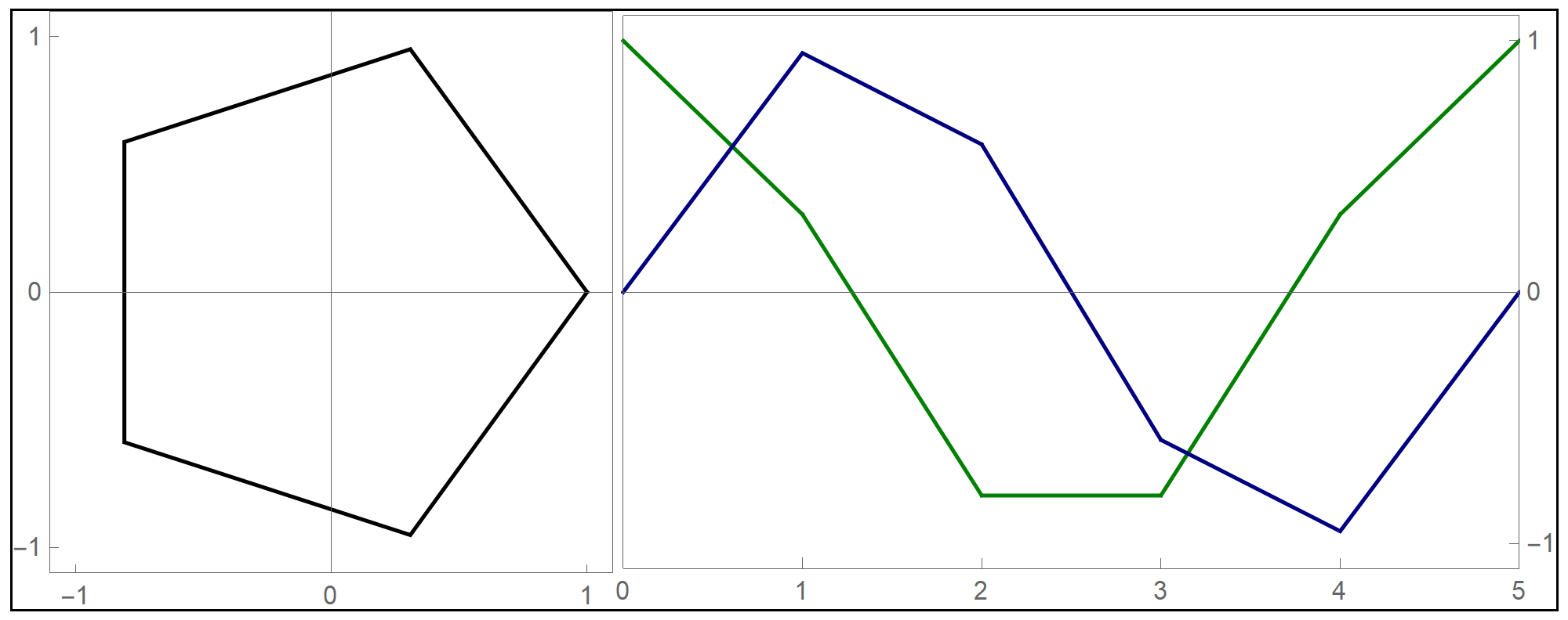
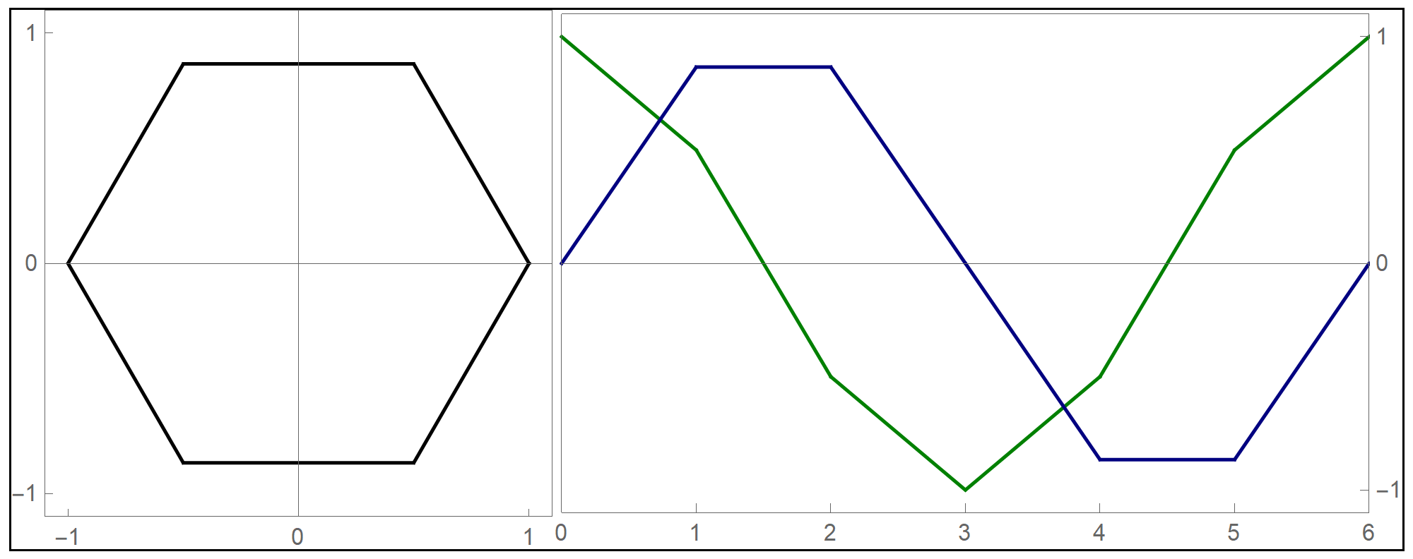
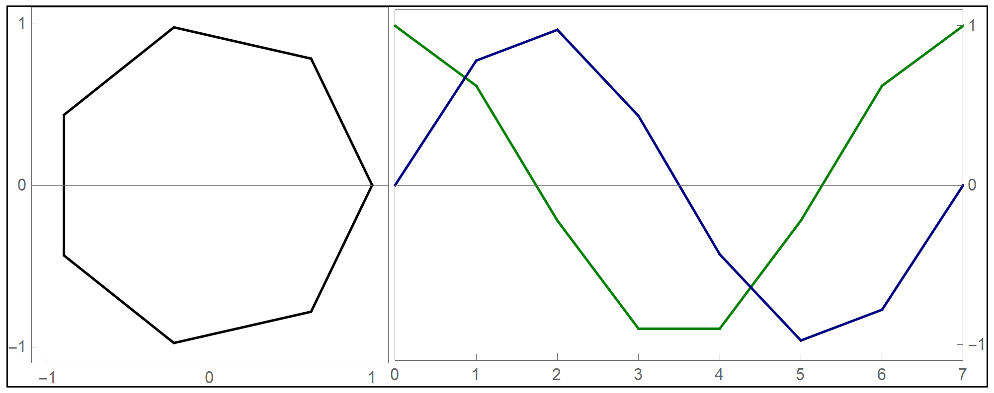
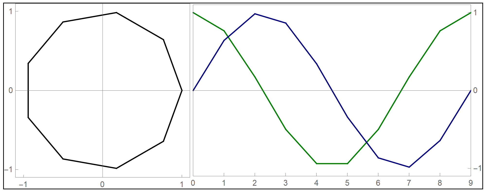
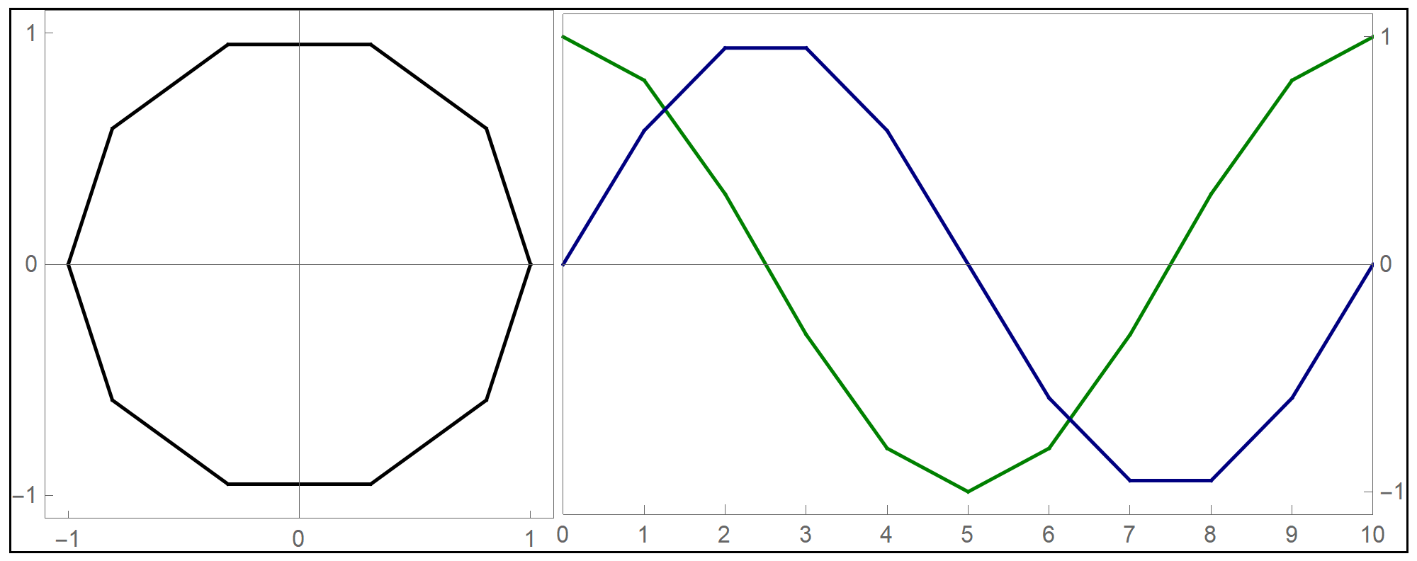
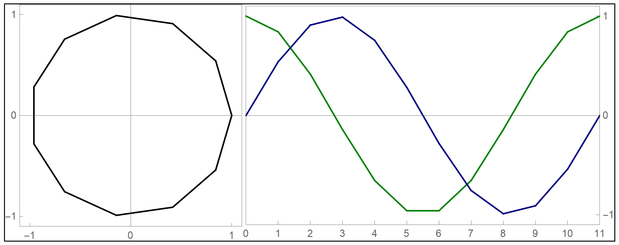
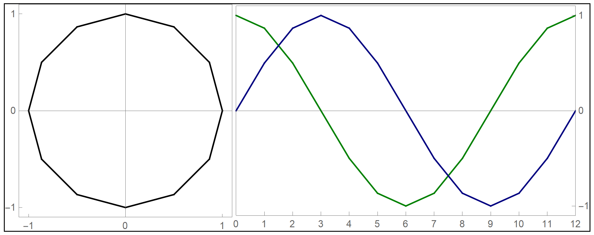
- I decided to test the general principle of parametric equations of curves in the plane on the example of regular \(n\)-gons inscribed in the unit circle: the equilateral triangle, square, regular pentagon, regular hexagon, regular heptagon, regular octagon, regular nonagon, regular decagon, regular hendecagon (or undecagon), regular dodecagon, and so on.
-
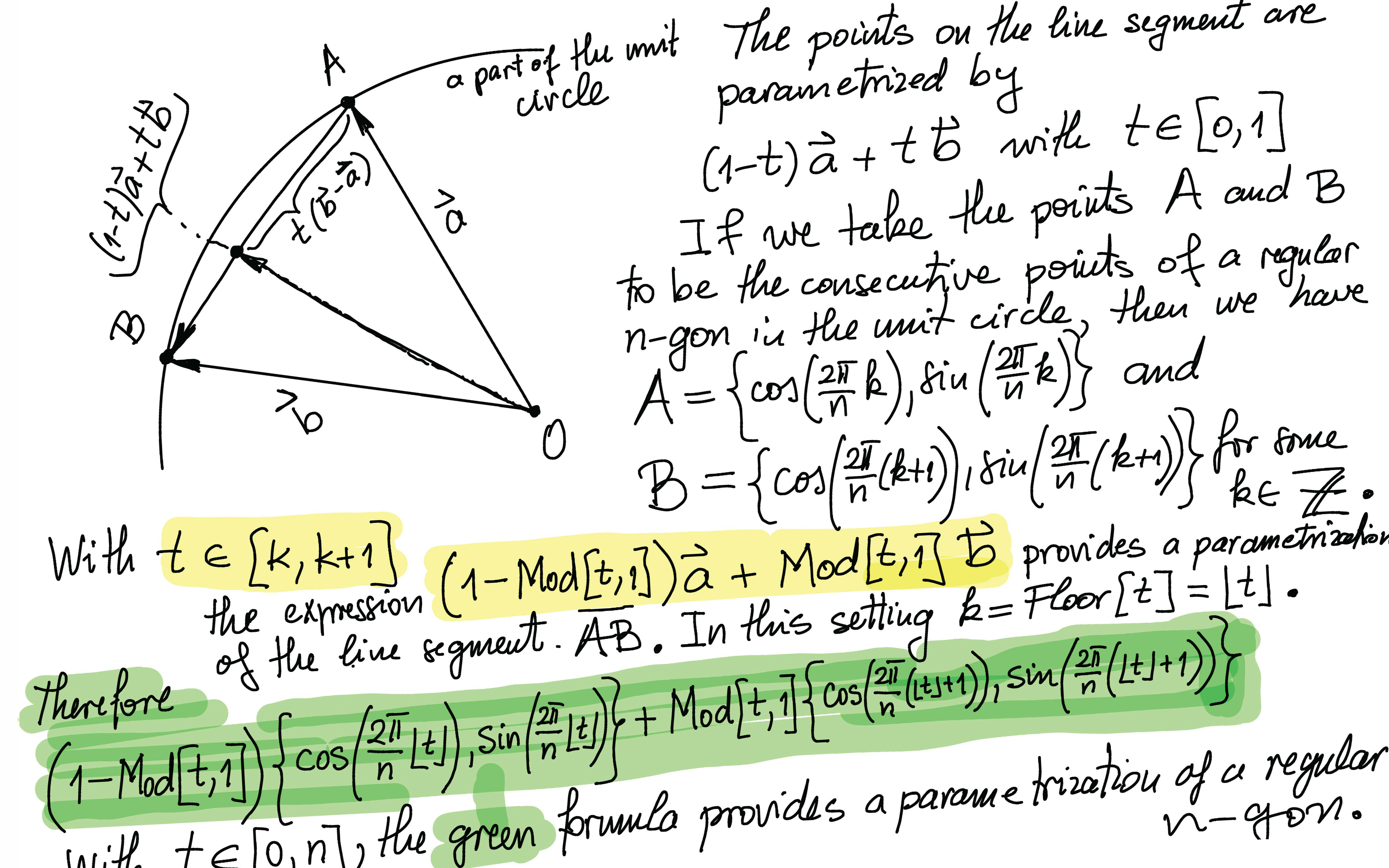
In the PNG picture below I explain the geometry that is behind the definition of
NgonCos[] and NgonSin[]
which I defined yesterday in class. In the PNG picture below I used the function
Mod[t,1]. It is just the function t - Floor[t].
-
The formulas derived in the preceding item, implemented in Mathematica are as follows:
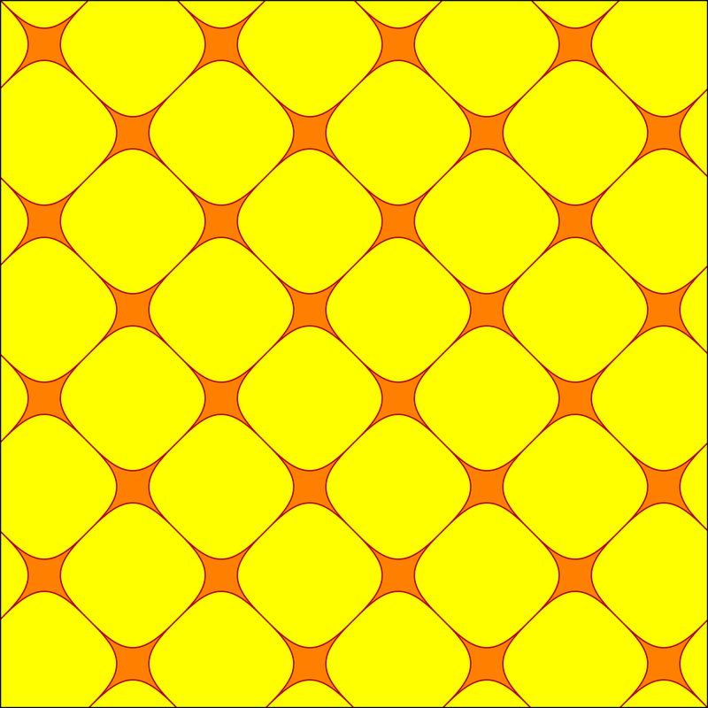
Clear[NgonCos, NgonSin, t, nn]; NgonCos[t_, nn_] := (1 - (t - Floor[t])) Cos[(2/nn) \[Pi] Floor[t]] + (t - Floor[t]) Cos[(2/nn) \[Pi] (1 + Floor[t])]; NgonSin[t_, nn_] := (1 - (t - Floor[t])) Sin[(2/nn) \[Pi] Floor[t]] + (t - Floor[t]) Sin[(2/nn) \[Pi] (1 + Floor[t])]; - The final product of this work are the graphs of the first nine regular $n$-gons inscribed in the unit circel: the equilateral triangle, the square, and the pentagon, the hexagon, the heptagon, the octagon, the nonagon, the decagon, the hendecagon, the dodecagon, see the Regular Polygon webpage at Wolfram MathWorld.
Hover over the image to start the animation.

- The information sheet (updated)
- We will use

- To get started with Mathematica see my Mathematica page. Please watch the videos that are on my Mathematica. Watching the movies is essential for being able to organize your homework notebooks well! I will not discuss the basics of notebook structuring in class.
- In the study of the computational software system Wolfram Mathematica, we will focus on symbolic and numerical calculations, visualization, and programming in Mathematica. But Mathematica is much more than that. To read more about Mathematica see An Elementary Introduction to the Wolfram Language.
-
As we begin the Mathematica portion of this class, a natural question arises: Why learn Mathematica? This is not an easy question to answer, but below are some key aspects that make Mathematica worth your attention.
- Mathematica is a powerful computational tool that can handle a wide range of mathematical problems, from basic algebra to advanced calculus and beyond.
- Unlike many other mathematical software systems, Mathematica excels in symbolic computation, allowing you to manipulate mathematical expressions and equations symbolically, closely resembling abstract mathematical thinking and structures.
- Mathematica offers powerful visualization tools, allowing you to create compelling graphics that enhance the understanding of mathematical concepts and effectively illustrate abstract mathematical results, fostering a varied and engaging mathematical learning experience.
- Mathematica is a high-level programming language that offers an extensive array of predefined functions, designed to simplify and streamline tasks that are commonly encountered in mathematical and technical computing. My impression is that this makes it more accessible and user-friendly compared to other mathematical software, enabling users to achieve complex objectives with greater ease.
- A lot of help is available on-line, for example Mathematica Stack Exchange, Wolfram Community and ChatGPT is quite good at offering help with Mathematica questions.
- Mathematica makes solving mathematical problems more efficient. How? For problems involving symbolic manipulation, we can perform symbolic manipulations in Mathematica exactly. For problems in which symbolic manipulations are inefficient, numerical approximations can be performed. Additionally, powerful graphical visualizations help guide the problem-solving process, offering deeper insights.
-
I have enjoyed the interaction between my mind and computers since I first started using them in the early 1990s. Recently, I came across a powerful metaphor for this relationship, expressed by Steve Jobs. In an old interview, he illustrated the usefulness of computers with a compelling analogy: "For me, a computer has always been a bicycle for the mind." That perfectly describes Mathematica and other modern tools like ChatGPT. Isn't that wonderful?
 See the Bicycle for the Mind video. Or, a longer
version.
See the Bicycle for the Mind video. Or, a longer
version.
- I am convinced that your mathematical learning experience will be enriched if you engage in mathematical explorations using technology.
-
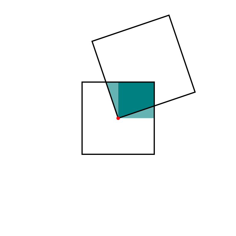
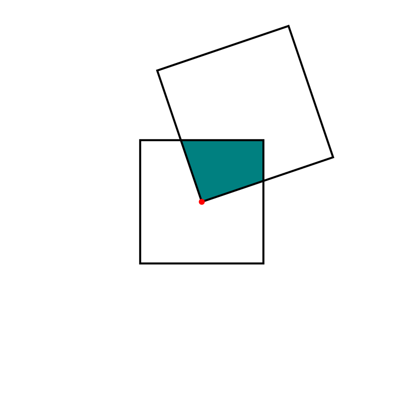
I recently encountered a fascinating geometric fact online: Imagine two squares where a vertex of the larger square is positioned at the center of the smaller square. Regardless of how these two squares are positioned, the area of their intersection remains constant. My description might not fully capture the beauty of this fact — indeed, an animation is worth a thousand words. How am I to make an animation? I must use technology. Here is an animation created in Mathematica.
Hover over the image to start the animation.
-
I should have left it as an exercise for you to figure out why what I claim in the preceding item is true. But, the solution supported by a Mathematica animation might indicate why using technology can be powerful tool in communicating Mathematics.
Hover over the image to start the animation.