- The most important concept for double integrals in polar coordinates is the area element in polar coordinates: $dA = r \, d\theta \, d r$.
-
The first step toward understanding spherical coordinates is understanding the unit vectors in $\mathbb{R}^3.$
- The importance of the trigonometric functions $\cos$ and $\sin$ is that each point on the unit circle in $\mathbb{R}^2$ can be expressed as $\bigl( \cos t, \sin t \bigr)$ with $t \in [0, 2\pi)$, or with $t\in (-\pi,\pi].$ This is the reason that trigonometric functions are also called circular functions.
- If we denote the coordinate unit vectors in $\mathbb{R}^2$ by $\boldsymbol{i}$ and $\boldsymbol{j},$ then each unit vector $\boldsymbol{u}$ in $\mathbb{R}^2$ can be expressed as \[ \boldsymbol{u} = (\cos \theta) \boldsymbol{i} + (\sin \theta) \boldsymbol{j}, \qquad \quad \theta \in [0,2 \pi). \]
-
Let now $\boldsymbol{v}$ be a unit vector in the three-dimensional space $\mathbb{R}^3.$ That is
\[
\boldsymbol{v} = v_1 \boldsymbol{i} + v_2 \boldsymbol{j} + v_3 \boldsymbol{k}.
\]
In the figure below the choice of colors is not random:
- $\boldsymbol{v}$ is the black vector;
- $\boldsymbol{i}$ is the red vector;
- $\boldsymbol{j}$ is the green vector;
- $\boldsymbol{k}$ is the blue vector;
- the yellow vector is the unit vector in the direction of the projection of $\boldsymbol{v}$ onto $xy$-plane. Say, as before, \[ \boldsymbol{u} = (\cos \theta) \boldsymbol{i} + (\sin \theta) \boldsymbol{j}, \qquad \quad \theta \in [0,2 \pi); \] The angle $\theta$ is also colored yellow.
- $\phi \in (0,\pi)$ is the gray angle between $\boldsymbol{v}$ and $\boldsymbol{k}$.
Click on the image to animate in $\theta$; double-click to animate in $\phi$.
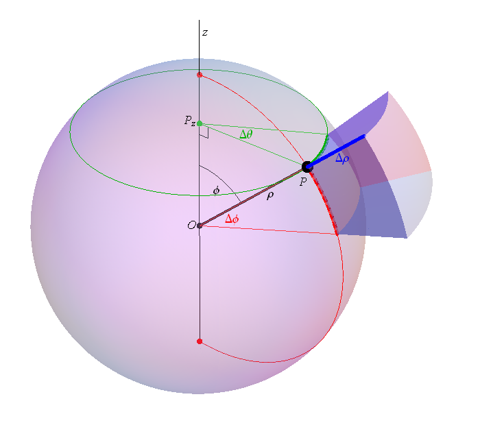
- In conclusion, each unit vector $\boldsymbol{v}$ in three-dimensional space is uniquely determined by two angles: the angle $\phi \in [0,\pi]$ between $\boldsymbol{v}$ and $\boldsymbol{k}$ and the angle $\theta \in [0,2 \pi)$ which is the angle between the projection of $\boldsymbol{v}$ onto $xy$-plane and $\boldsymbol{i}$. Then \[ \boldsymbol{v} = (\sin \phi)(\cos \theta) \boldsymbol{i} + (\sin \phi)(\sin \theta) \boldsymbol{j} + (\cos \phi) \boldsymbol{k}. \]
-
To enrich our toolbox for calculating triple integrals we need to understand cylindrical and spherical coordinates. The most important concepts here are the volume element in cylindrical coordinates: $dV = r \, d\theta \, d r \, dz$ and
the volume element in spherical coordinates is: $dV = \rho^2 (\sin \phi) \, d\theta\, d\phi \, d\rho$. I created the image below to help you understand this formula.
-
In the problems below I use the following notation. The unit disk in $\mathbb{R}^2$ is denoted by $\mathbb{D}$. That is
\[
\mathbb{D} = \bigl\{ (x,y) \in \mathbb{R}^2 \ \vert \ x^2 + y^2 \leq 1 \bigr\}.
\]
The special square in $\mathbb{R}^2$ whose edges are tangent to $ \mathbb{D}$ and parallel to the coordinate axes is denoted by $\mathbb{Q}$. That is,
\[
\mathbb{S} = \bigl\{ (x,y) \in \mathbb{R}^2 \ \vert \ x,y \in [-1,1] \bigr\}.
\]
The unit ball in $\mathbb{R}^3$ is denoted by $\mathbb{B}$. That is
\[
\mathbb{B} = \bigl\{ (x,y,z) \in \mathbb{R}^3 \ \vert \ x^2 + y^2 + z^2 \leq 1 \bigr\}.
\]
The special cube in $\mathbb{R}^3$ whose sides are tangent to $\mathbb{B}$ and parallel to the coordinate planes is denoted by $\mathbb{U}$. That is,
\[
\mathbb{U} = \bigl\{ (x,y,z) \in \mathbb{R}^3 \ \vert \ x,y,z \in [-1,1] \bigr\}.
\]
- Problem 1. Find the average distance of a point in $\mathbb{D}$ to the center $(0,0)$ of $\mathbb{D}.$
- Problem 2. Find the average distance of a point in $\mathbb{D}$ to a fixed diameter of $\mathbb{D}.$ Here you can choose a diameter along the $x$-axis or along the $y$-axis.
- Problem 3. Find the average distance of a point in $\mathbb{D}$ to the coordinate axes. Recall that the distance of a point $(x,y)$ to the coordinate axes is given by $\min\{|x|,|y|\}.$
- Problem 4. Find the average distance of a point in $\mathbb{S}$ to the $x$-axis.
- Problem 5. Find the average distance of a point in $\mathbb{S}$ to a fixed diagonal of $\mathbb{S}.$ Here you can choose the diagonal joining the points $(-1,-1)$ and $(1,1).$
- Problem 6. Find the average distance of a point in $\mathbb{S}$ to the coordinate axes.
- Problem 7. Find the average distance of a point in $\mathbb{B}$ to the center $(0,0,0)$ of $\mathbb{B}.$
- Problem 8. Find the average distance of a point in $\mathbb{B}$ to a fixed diameter of $\mathbb{B}.$ Here you can chose the diameter along the $z$-axis.
- Problem 9. Find the average distance of a point in $\mathbb{B}$ to $xy$-plane.
- Problem 10. Find the average distance of a point in $\mathbb{B}$ to the coordinate planes. Recall that the distance of a point $(x,y,z)$ to the coordinate planes is given by $\min\{|x|,|y|,|z|\}.$ (This is the hardest problem on this list.)
- Problem 11. Find the average distance of a point in $\mathbb{U}$ to $xy$-plane.
- Problem 12. Find the average distance of a point in $\mathbb{U}$ to the coordinate planes.
-
Today we started Section 5.5 Triple Integrals in Cylindrical and Spherical Coordinates in OpenStax Calculus Volume 3. Do as many problems from 241 to 296 as you can. In particular: 243, 244, 245, 260, 261, 262, 263, 271, 272, .
-
Today we started Section 5.4 Triple Integrals in OpenStax Calculus Volume 3. Do as many problems from 181 to 240 as you can. In particular: 182, 189, 191, 194, 198, 209, 211, 212, 219, 221, 222, 223, 229, 231, 232, 235, 236, 237, 239.
-
Today we started Section 5.3 Double Integrals in Polar Coordinates in OpenStax Calculus Volume 3. Do as many problems from 122 to 180 as you can. In particular: 123, 125, 126, 127, 129, 131, 131, 132, 134, 135, 140, 144, 145, 146, 147, 150, 153, 157, 160, 178.
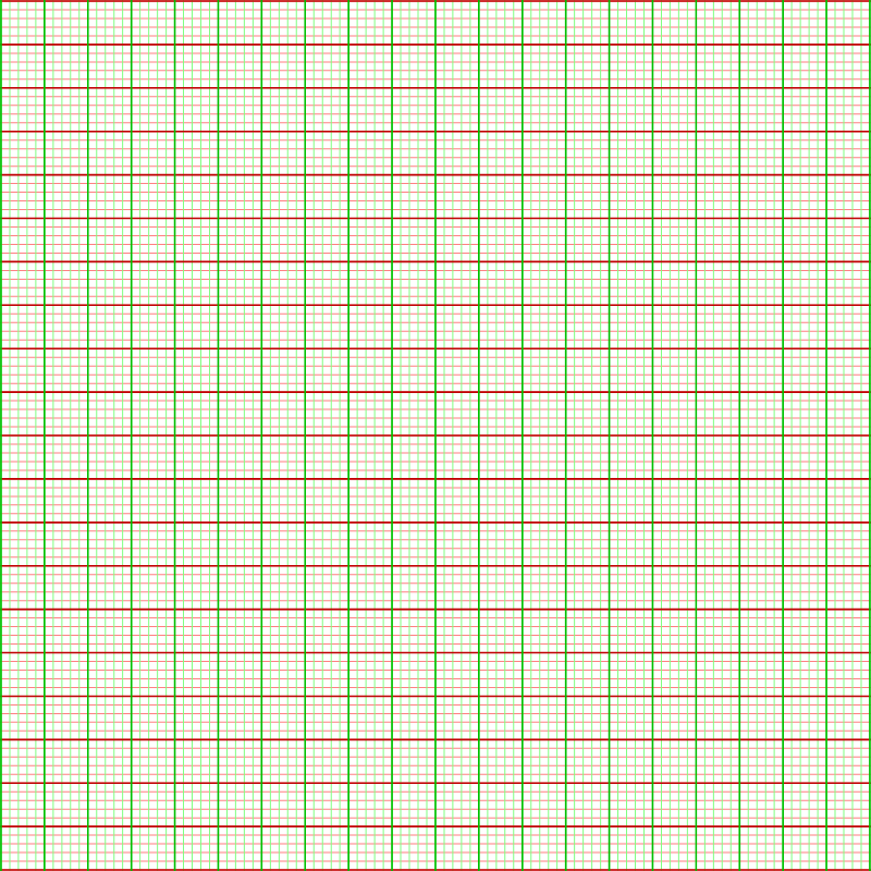
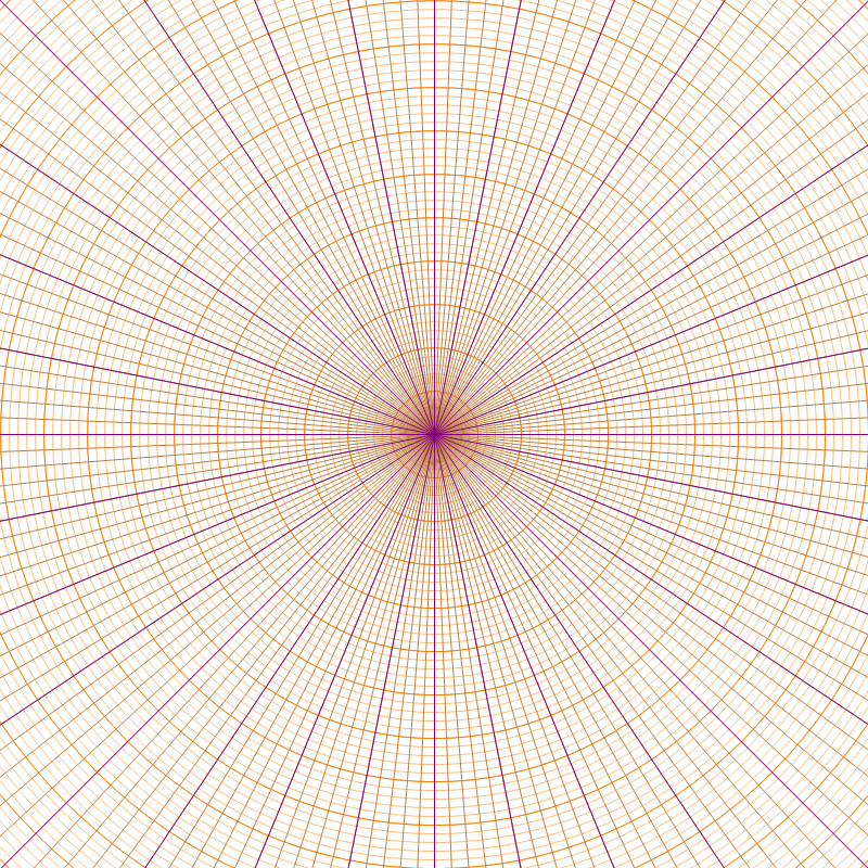
- I just could not resist producing a fine Cartesian and a fine polar grid.
-
Today we started Section 5.2 Double Integrals over General Regions in OpenStax Calculus Volume 3. Do as many problems from 60 to 121 as you can. In particular: 61, 64, 69, 77, 86, 87, 94, 100, 109, 111, 114, 115, 120 (this is not a "technology" problem), 121.
-
Today we did Section 5.1 Volumes and Double Integrals in OpenStax Calculus Volume 3. Do as many problems from 1 to 59 as you can. In particular: 2, 4, 6, 9, 11, 12, 17, 25, 26, 27, 28, 30, 33, 35, 36, (38 involves a very difficult integral), 39, 51, 52.
-
In this item I present some properties of the cords and triangles in the unit circle.
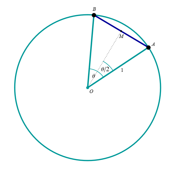
Cord length 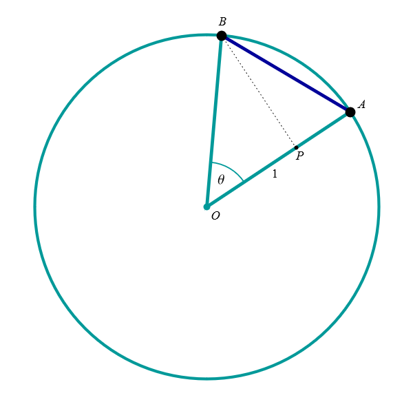
Area of central triangle Calculating length of a cord. In the figure with the capture "Cord length" you can see how the length of the cord \(\overline{AB}\) in the unit circle is expressed in terms of the central angle \(\theta,\) where \(\theta \in (0,\pi),\) that is \(\theta\) is an angle less than \(\pi.\) The length of \(\overline{AB}\) is equal to \(2 \sin(\theta/2).\) To prove this claim mark by \(M\) the midpoint of the cord \(\overline{AB}.\) Then the line \(OM\) is orthogonal to the line \(AB\) and the angle \(\measuredangle MOA\) is equal to \(\theta/2.\) Since the length of the line segment \(\overline{OM}\) is \(1,\) the length of \(\overline{AM}\) is \(\sin(\theta/2).\) Since \(M\) is the midpoint of the cord \(\overline{AB},\) the length of \(\overline{AB}\) is \(2 \sin(\theta/2).\) Looking at this formula, we notice that it is also valid for \(\theta = 0,\) when the cord is just a point, and for \(\theta = \pi\) when the cord is a diameter.
Calculating area of a central triangle. In the figure with the capture "Area of central triangle with vectors" you can see how to express the area of a central triangle \(\triangle OAB\) in the unit circle is expressed in terms of the central angle \(\theta,\) where \(\theta \in (0,\pi),\) that is \(\theta\) is an angle less than \(\pi.\) The area of the triangle \(\triangle OAB\) is equal to \(\sin(\theta).\) To prove this claim mark by \(P\) the point on the radius \(\overline{OA}\) such that the line \(BP\) is orthogonal to \(OA.\) Then the line segment \(\overline{BP}\) is the height of the triangle \(\triangle OAB.\) Since the triangle \(\triangle OPB\) is the right triangle with the hypothenus of length \(1,\) the length of \(\overline{BP}\) is \(\sin(\theta).\) Thus, the base of \(\triangle OAB\) is \(\overline{OA}\) of lenght \(1\) and the length of the corresponding height \(\overline{BP}\) is \(\sin(\theta),\) the area of \(\triangle OAB\) is \(\tfrac{1}{2}\sin(\theta).\) Looking at this formula, we notice that it is also valid for \(\theta = 0,\) when the triangle is degenerates to a radius with area \(0\), and for \(\theta = \pi\) when the triangle degenerates to a diameter with area \(0.\)
-
Positioning of a triangle inscribed in the unit circle. Every triangle inscribed in the unit circle can be rotated so that one vertex is at the point \((1,0),\) and one of the remaining vertices is above, and the other one below the horizontal diameter. If the triangle is obtuse or right, the vertex corresponding to the obtuse or right angle is rotated to the point \((1,0).\) If the triangle is acute, any vertex can be rotated to \((1,0).\) The four pictures below illustrate this claim.
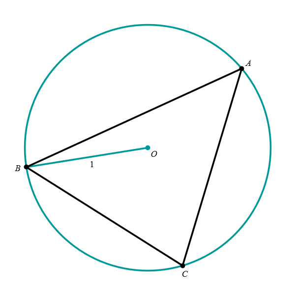
Acute triangle 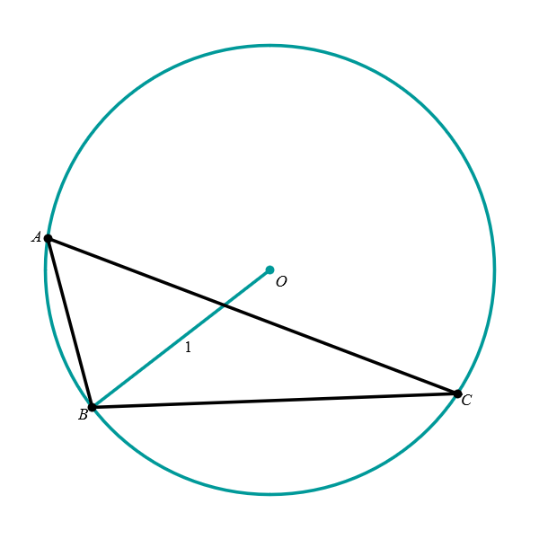
Obtuse triangle 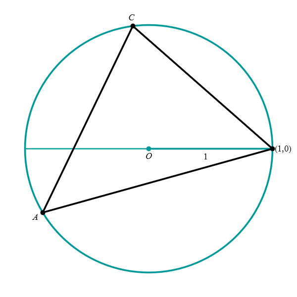
Rotated acute triangle 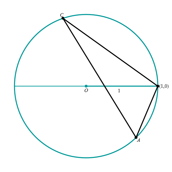
Rotated obtuse triangle -
Problem. Among all triangles inscribed in the unit circle find those with the maximum perimeter.
Solution. Step I: Finding the function to optimize. It follows from the discussion in "Positioning of a triangle inscribed in the unit circle" that we can consider only triangles with one vertex at \((1,0)\) and the other two vertices on opposite sides of the horizontal diameter. Thus, there exist \(\alpha, \beta \in (0,\pi)\) such that the vertices of the triangle are \[ \bigl( \cos\alpha, \sin\alpha\bigr), \quad (1,0), \quad \bigl( \cos\beta, -\sin\beta\bigr). \] See the pictures below.
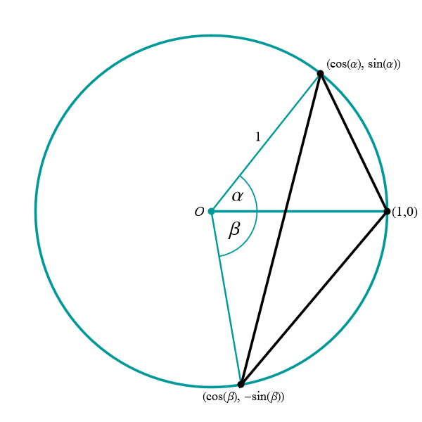
Obtuse triangle 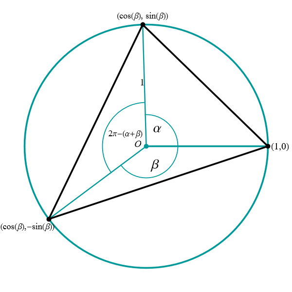
Acute triangle Now we calculate the perimeter in each case. Notice that both angles \(\alpha\) and \(\beta\) are positive.
Looking at the obtuse triangle, we see that all the angles \(\alpha,\) \(\beta,\) and \(\alpha+\beta\) are less or equal to \(\pi.\) Using the result from calculating length of a cord, the length of the cord connecting the points $\bigl( \cos\alpha, \sin\alpha\bigr)$ and $(1,0)$ is \(2 \sin(\alpha/2).\) The length of the cord connecting the points $\bigl( \cos\beta, -\sin\beta \bigr)$ and $(1,0)$ is \(2 \sin(\beta/2).\) The length of the cord connecting the points $\bigl( \cos\beta, -\sin\beta \bigr)$ and $\bigl( \cos\alpha, \sin\alpha\bigr)$ is \(2 \sin\bigl((\alpha+\beta)/2\bigr).\) Thus the perimeter is \[ 2 \Bigl( \sin\bigl(\alpha/2\bigr) + \sin\bigl(\beta/2\bigr) + \sin\bigl((\alpha+\beta)/2\bigr) \Bigr). \]
Looking at the acute triangle, we see that the angles \(\alpha\) and \(\beta\) are less than \(\pi\) and that the angle \(\alpha+\beta\) is greater than \(\pi.\) Using the result from calculating length of a cord, the length of the cord connecting the points $\bigl( \cos\alpha, \sin\alpha\bigr)$ and $(1,0)$ is \(2 \sin(\alpha/2).\) The length of the cord connecting the points $\bigl( \cos\beta, -\sin\beta \bigr)$ and $(1,0)$ is \(2 \sin(\beta/2).\) In this case, the length of the cord connecting the points $\bigl( \cos\beta, -\sin\beta \bigr)$ and $\bigl( \cos\alpha, \sin\alpha\bigr)$ is \[ 2 \sin\Bigl( \frac{2\pi - (\alpha+\beta)}{2} \Bigr) = 2 \sin\Bigl( \pi - \frac{\alpha+\beta}{2} \Bigr) = 2 \sin\Bigl( \frac{\alpha+\beta}{2} \Bigr). \] Thus in this case the perimeter is also given by \[ 2 \Bigl( \sin\bigl(\alpha/2\bigr) + \sin\bigl(\beta/2\bigr) + \sin\bigl((\alpha+\beta)/2\bigr) \Bigr). \]
Step II: Finding the maximum. To find the triangle with the maximum perimeter, we need to find the maximum of the function \[ F(\alpha, \beta) = 2 \Bigl( \sin\bigl(\alpha/2\bigr) + \sin\bigl(\beta/2\bigr) + \sin\bigl((\alpha+\beta)/2\bigr) \Bigr), \quad \alpha, \beta \in [0,\pi]. \] We find critical points: \begin{align*} F_{\alpha}(\alpha, \beta) & = \cos\bigl(\alpha/2\bigr) + \cos\bigl((\alpha+\beta)/2\bigr) = 0,\\ F_{\beta}(\alpha, \beta) & = \cos\bigl(\beta/2\bigr) + \cos\bigl((\alpha+\beta)/2\bigr) = 0. \end{align*} Hence \[ \cos\bigl(\alpha/2\bigr) = \cos\bigl(\beta/2\bigr). \] Since \(\alpha/2 \in [0,\pi/2]\) and \(\beta/2 \in [0,\pi/2]\) we can apply the \(arccos\) function to get \[ \alpha/2 = \arccos \bigl( \cos\bigl(\alpha/2\bigr) \bigr) = \arccos\bigl( \cos\bigl(\beta/2\bigr)\bigr) = \beta/2. \] Hence \(\alpha = \beta.\) To determine the critical point we substitute \(\alpha = \beta\) in \[ \cos\bigl(\alpha/2\bigr) + \cos\bigl((\alpha+\beta)/2\bigr) = 0 \] to get \[ \cos\bigl(\alpha/2\bigr) + \cos\bigl(\alpha\bigr) = 0. \] To solve this equation one needs the double angle identity for the cosine function \[ \cos(2x) = (\cos x)^2 - (\sin x)^2 = (\cos x)^2 - \bigl( 1 - (\cos x)^2 \bigr) = 2 (\cos x)^2 - 1 \] Hence, with \(x = \alpha/2\) we have \[ \cos\bigl(\alpha/2\bigr) + 2 \bigl(\cos\bigl(\alpha/2\bigr)\bigr)^2 - 1 = 0. \] Since \(\cos\bigl(\alpha/2\bigr) \gt 0,\) the solution is \[ \cos\bigl(\alpha/2\bigr) = \frac{1}{2}, \quad \text{that is} \quad \frac{\alpha}{2} = \frac{\pi}{3}. \] Thus, the only critical point is \[ \alpha = \frac{2\pi}{3}, \quad \beta = \frac{2\pi}{3}. \]
Going back to the meaning of the angles \(\alpha\) and \(\beta\) we see that \[ \alpha = \frac{2\pi}{3}, \quad \beta = \frac{2\pi}{3}. \] give the equilateral triangle. Thus, the triangle with the maximum perimeter inscribed in the unit circle is the equilateral triangle.
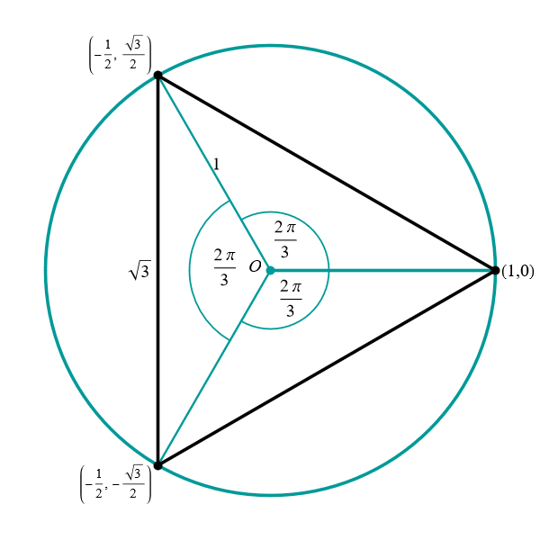
The equilateral triangle 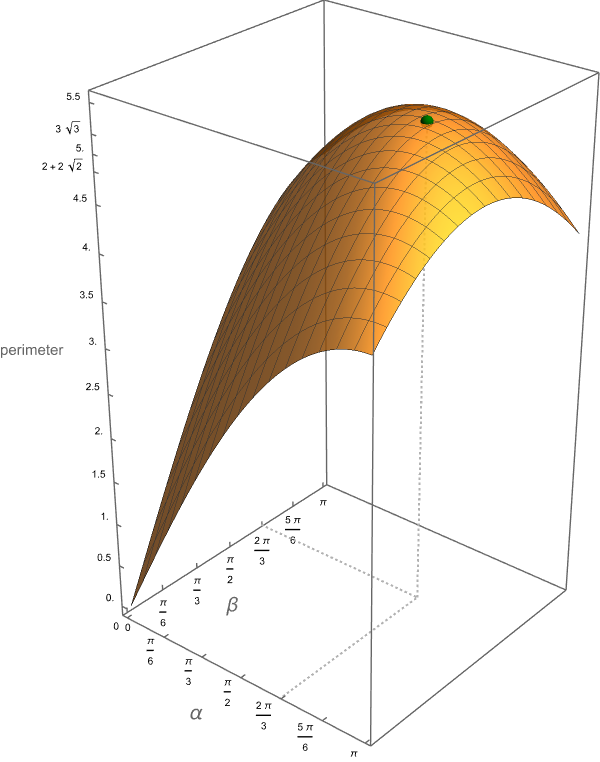
The graph of the perimeter function -
The right triangle with \(\alpha= \pi, \beta=\pi/2\) attracted my attention. The perimeter of this triangle is \(2+2\sqrt{2}.\) There are many other triangles with the same perimeter. On the graph of the perimeter function below, I emphasized the level curve \[ 2 \Bigl( \sin\bigl(\alpha/2\bigr) + \sin\bigl(\beta/2\bigr) + \sin\bigl((\alpha+\beta)/2\bigr) \Bigr) = 2+2\sqrt{2}. \] In the \(\alpha\beta\)-plane I emphasized all the pairs \((\alpha,\beta)\) which result in the triangles with the perimeter \(2+2\sqrt{2}.\) Three such pairs are given below \[ \bigl(\pi, \pi/2\bigr), \quad \bigl(\pi/2, \pi/2\bigr), \quad \bigl(\pi/2, \pi\bigr). \]
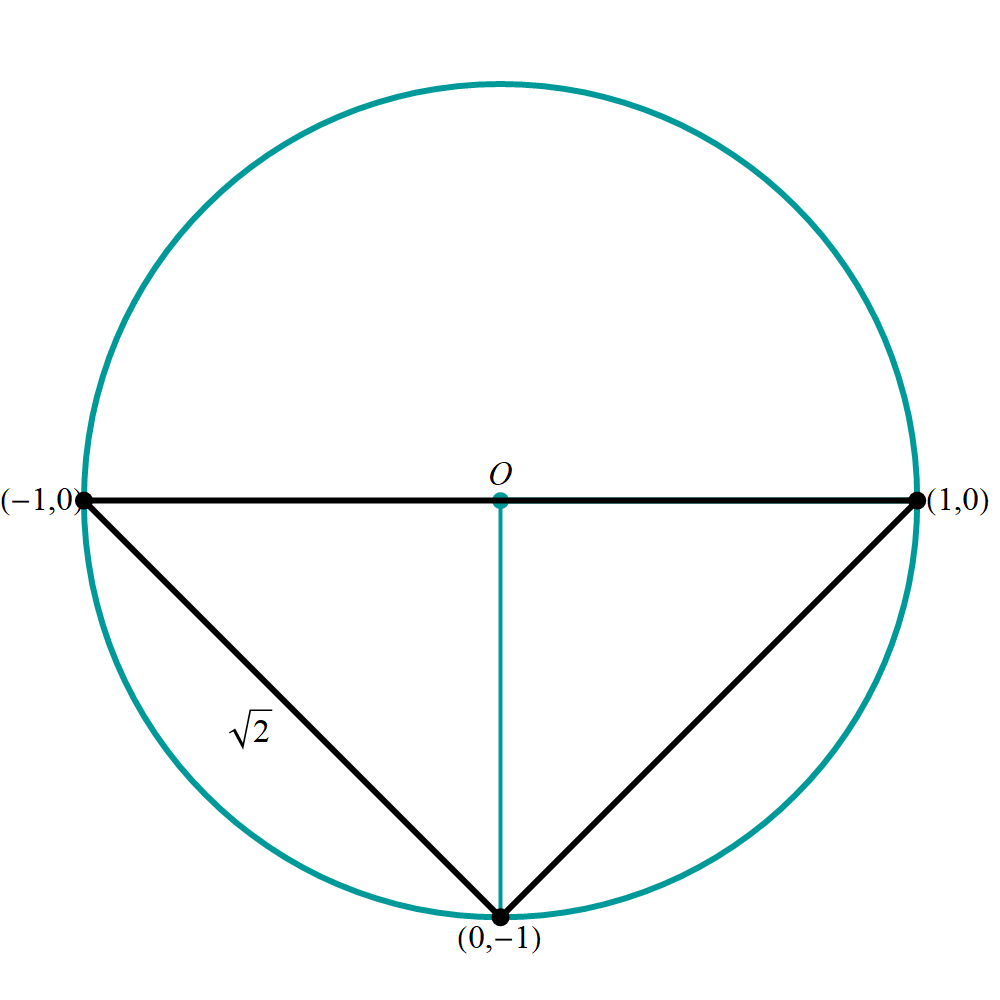
The right triangle \(\alpha= \pi, \beta=\pi/2\) 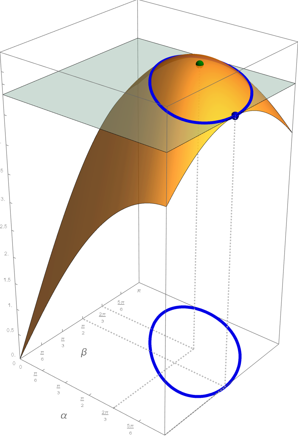
The graph of the perimeter function However, as we can see from the plot of the level curve there are infinitely many triangles with the perimeter \(2+2\sqrt{2}.\) In collaboration with ChatGPT, I wrote Wolfram Mathematica code to give me 207 pairs of the angles \(\alpha\) and \(\beta\) for triangles with the perimeter \(2+2\sqrt{2}.\) The resulting animation is below.
Place the cursor over the image to start the animation.
-
Problem. Among all triangles inscribed in the unit circle find those with the maximum area.
Solution.
-
Problem. Find the cuboid of maximum volume whose one vertex is at the origin, the cross diagonal vertex \((x,y,z)\) is on the ellipsoid \(x^2 + 2 y^2 + 3 z^2 = 6\) with all \(x,y,z \gt 0\) and whose sides are parallel to the coordinate planes.
Solution. In this problem we need to maximize the function \(f(x,y,z) = xyz\) subject to the constrained \(g(x,y,z) = x^2 + 2 y^2 + 3 z^2 - 6 = 0\) and \(x,y,z \gt 0.\) This is a clear application of the method of Lagrange multipliers.
First we calculate the gradient vectors \[ \begin{aligned} (\boldsymbol{\nabla} f)(x,y,z) & = \Bigl\langle yz, xz, xy \Bigr\rangle \\ (\boldsymbol{\nabla} g)(x,y,z) & = \Bigl\langle 2x, 4y, 6z \Bigr\rangle \end{aligned} \] The maximum will be at the point \((x,y,z)\) that satisfies the equations \(g(x,y,z) = x^2 + 2 y^2 + 3 z^2 - 6 = 0\) and \((\boldsymbol{\nabla} f)(x,y,z) = \lambda (\boldsymbol{\nabla} g)(x,y,z)\) and \(x,y,z \gt 0.\) That is we need to solve the system \[ \begin{aligned} y z& = 2\lambda x \\ xz & = 4\lambda y \\ xy & = 6\lambda z \\ x^2 + 2 y^2 + 3 z^2 & = 6 . \end{aligned} \]
We solve the first three equations multiply by the missing variable on the left-hand side: \begin{align*} yz = 2\lambda x \quad &\implies \quad xyz = 2\lambda x^2 \\ xz = 4\lambda y \quad &\implies \quad xyz = 4\lambda y^2 \\ xy = 6\lambda z \quad &\implies \quad xyz = 6\lambda z^2 \end{align*} Since we are given that $x, y, z > 0$, the volume $V = xyz$ must be positive. This implies that $\lambda \gt 0$. Therefore \[ \frac{xyz}{\lambda} = 2 x^2 = 4 y^2 = 6 z^2. \] Now we can express $y^2$ and $z^2$ in terms of $x^2$: \begin{align*} y^2 &= \frac{1}{2}x^2 \\ z^2 &= \frac{1}{3}x^2 \end{align*}
Substitute these relationships into the constraint equation: $$ x^2 + 2\left(\frac{1}{2}x^2\right) + 3\left(\frac{1}{3}x^2\right) = 6 $$ $$ x^2 + x^2 + x^2 = 6 $$ $$ 3x^2 = 6 $$ $$ x^2 = 2 $$ Since $x > 0$, we have $x = \sqrt{2}$. Now we find the corresponding $y$ and $z$ values: \begin{align*} y^2 &= \frac{1}{2}x^2 = \frac{1}{2}(2) = 1 \quad \implies \quad y = 1 \quad (\text{since } y > 0) \\ z^2 &= \frac{1}{3}x^2 = \frac{1}{3}(2) = \frac{2}{3} \quad \implies \quad z = \sqrt{\frac{2}{3}} = \frac{\sqrt{6}}{3} \quad (\text{since } z > 0) \end{align*} The vertex on the ellipsoid that maximizes the volume is $\left(\sqrt{2}, 1, \sqrt{\frac{2}{3}}\right)$.
The maximum volume $V$ is the product of these coordinates: $$ V = xyz = (\sqrt{2}) \cdot (1) \cdot \left(\sqrt{\frac{2}{3}}\right) = \frac{2}{\sqrt{3}} = \frac{2\sqrt{3}}{3}.$$
The maximum volume of the cuboid is $\frac{2\sqrt{3}}{3}$, which occurs when the vertex on the ellipsoid is at the point $\left(\sqrt{2}, 1, \frac{\sqrt{6}}{3}\right)$.
Let us verify one other point on the ellipsoid, for example $\left(2, 1/2, \frac{\sqrt{2}}{2}\right).$ The corresponding volume is \(\displaystyle \frac{\sqrt{2}}{2}.\) Since \[ \frac{\sqrt{2}}{2} \lt 1 \qquad \text{and} \qquad 1 \lt \frac{2\sqrt{3}}{3}, \] this is consistent with our claim that we have found the cuboid with the maximum volume. These two cuboids are illustrated in the picture below.
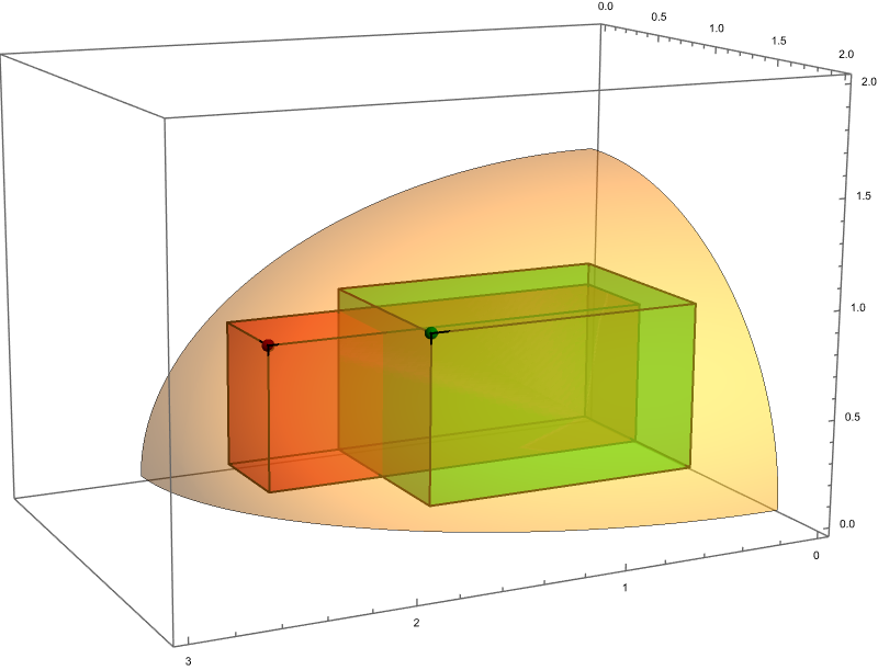
Below is Wolfram Mathematica code for the above plot.
Show[ContourPlot3D[ x^2 + 2 y^2 + 3 z^2 == 6, {x, 0, 3}, {y, 0, 2}, {z, 0, 2}, Mesh -> False, PlotPoints -> {100, 100, 100}, ContourStyle -> Directive[Opacity[0.5]]], Graphics3D[{{RGBColor[0, 0.5, 0], Sphere[{Sqrt[2], 1, Sqrt[2/3]}, 0.03], RGBColor[0.5, 0, 0], Sphere[{2, 1/2, Sqrt[1/2]}, 0.03]}, {Opacity[0.5], EdgeForm[Thick], FaceForm[Green], Cuboid[{0, 0, 0}, {Sqrt[2], 1, Sqrt[2/3]}]}, {Opacity[0.5], EdgeForm[Thick], FaceForm[Red], Cuboid[{0, 0, 0}, {2, 1/2, Sqrt[1/2]}]}}], BoxRatios -> {3, 2, 2}, PlotRange -> {{0, 3}, {0, 2}, {0, 2}}, ImageSize -> 800, ViewPoint -> {1.475939270706893`, 2.9493993057214207`, 0.7567344346567079`}, ViewVertical -> {0.14219484790908707`, 0.41320353056636794`, 0.8994684361085719`}, ViewCenter -> {0.5`, 0.5`, 0.5`}, ViewAngle -> Automatic, ViewVector -> Automatic, ViewMatrix -> Automatic, ViewRange -> All] -
Problem. Find a triangle inscribed in the unit circle with the maximum perimeter.
Solution. In this problem we need to maximize the function \(f(x,y,z) = xyz\) subject to the constrained \(g(x,y,z) = x^2 + 2 y^2 + 3 z^2 - 6 = 0\) and \(x,y,z \gt 0.\) This is a clear application of the method of Lagrange multipliers.
-
Today we did Section 4.8 Lagrange Multipliers in OpenStax Calculus Volume 3. Do as many problems from 358 to 393 as you can. In particular: 358, 359, 365, 371, 377, 380, 381, 382, 383 (is wrong, probably should be "on the curve in \(xy\)-plane"), 384 (probably does not belong to this section, but it is a nice problem), 391, 392.
-
Today in class, I found the axes of the ellipse given by \(2 x^2 - 4 x y + 5 y^2 = 12.\) I used this example to introduce the method of Lagrange multipliers. The motivation comes from the picture below: the purple circles centered at the origin help identify the points on the blue ellipse that are closest to and farthest from the origin.
The key idea is to recognize the gradients of the two functions:
- $f(x,y) = x^2 + y^2$ — the function we want to minimize or maximize (distance squared from the origin)
- $g(x,y) = 2x^2 - 4xy + 5y^2 - 12$ — the constraint defining the ellipse
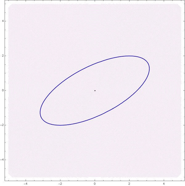
Below is Wolfram Mathematica code for the above plot.
Show[ContourPlot[2 x^2 - 4 x y + 5 y^2 == 12, {x, -5, 5}, {y, -5, 5},
  ContourStyle ->
   Directive[RGBColor[0.75 {0, 0, 1}], Thickness[0.003]]],
 ContourPlot[Sqrt[x^2 + y^2], {x, -5, 5}, {y, -5, 5},
  ContourShading -> False, Contours -> 150,
  ContourStyle ->
   Directive[Opacity[0.3], RGBColor[0.5 {1, 0, 1}],
    Thickness[0.001]]], Graphics[{Point[{0, 0}]}], ImageSize -> 600]
- Today I am posting an optimization problem related to an important mathematical inequality between the geometric and arithmetic means. The simplest version is a Calculus I problem. These problems are very similar to the problems that we discussed in class. I will formulate them as mathematical problems, without wrapping them in stories about fencing sheep, minimizing the surface area of a cuboid with fixed volume, or, even more ambitiously, trying to invent a story for a four-dimensional problem.
-
Problem. Let \(x\) and \(y\) be positive real numbers such that \(xy = 1.\) Under this condition, find the extreme value of the sum \(x+y\).
Solution. Let \(x\) and \(y\) be positive real numbers such that \(xy = 1.\) To find the extreme value of \(x+y\) we solve \(xy = 1\) for \(y = 1/x\) and consider \(x+y = x +1/x\) which is a function of one independent variable \(f(x) = x + 1/x.\) Clearly we can take \(x\) to be any large positive number and then \(f(x) \gt x.\) Therefore, \(f(x) = x + 1/x\) does not have a maximum. We use the first and second derivative to find and analyze critical points: \[ f'(x) = 1 - \frac{1}{x^2}, \qquad f''(x) = 2 \frac{1}{x^3} \gt 0. \] Therefore, \(f(x)\) has only one critical point \(x = 1\) and that critical point is local minimum, \(f(1) = 2.\) Since the second derivative is positive, the local minimum \(f(1) = 2\) is the global minimum. Therefore, \[ x + \frac{1}{x} \geq 2, \] for all positive real numbers \(x,\) and \[ x + \frac{1}{x} = 2 \quad \text{if and only if} \quad x = 1. \]
In the terminology of our original question, we proved the following statement: If \(x\) and \(y\) are positive real numbers such that \(xy = 1,\) then \(x+y \geq 2.\) The equality \(x+y = 2\) holds if and only if \(x = y =1.\)
-
Problem. Let \(x, y\) and \(z\) be positive real numbers such that \(xyz = 1.\) Under this condition, find the extreme value of the sum \(x+y+z\).
Solution. Let \(x, y\) and \(z\) be positive real numbers such that \(xyz = 1.\) To find the extreme value of \(x+y+z\) we solve \(xyz = 1\) for \(z = 1/(xy)\) and consider \(x+y+z = x + y + 1/(xy),\) which is a function of two independent variables \[ F(x,y) = x+y+ \frac{1}{xy}. \] Let us find the partial derivatives of this function \[ F_x(x,y) = 1 - \frac{1}{x^2 y}, \quad F_y(x,y) = 1 - \frac{1}{y^2 x}. \] and solve to find the critical points \[ 1 - \frac{1}{x^2 y} = 0, \quad 1 - \frac{1}{y^2 x} = 0. \] Therefore, \(x^2 y = y^2 x\) and consequently, \(x = y.\) Thus, the only critical point is \(x = 1, y= 1.\)
To find the discriminant at this critical point we calculate \[ F_{xx}(x,y) = \frac{2}{x^3 y}, \quad F_{yy}(x,y) = \frac{2}{y^3 x}, \quad F_{xy}(x,y) = \frac{1}{x^2 y^2}, \] evaluated at \(x = 1, y= 1\) to be \(F_{xx}(1,1) = 2,\) \(F_{yy}(1,1) = 2,\) and \(F_{xy}(1,1) = 1.\) Thus, the discriminant is \(2\cdot 2 - 1^2 = 3,\) and the critical point \(x = 1, y= 1\) is a local minimum, \[ F(1,1) = 1+1+ \frac{1}{1} = 3. \]
Next we will prove that this local minimum is global. That is we will prove \[ x + y + \frac{1}{xy} \geq 3 \quad \text{for all} \quad x, y \gt 0. \]
The argument uses the result of our first problem as follows: \[ x + y + \frac{1}{xy} = x + \frac{1}{\sqrt{x}} \Bigl( y \sqrt{x} + \frac{\sqrt{x}}{xy} \Bigr). \] Why I use this factorization? Amazingly, the sum in the big parenthesis \[ \Bigl( y \sqrt{x} + \frac{\sqrt{x}}{xy} \Bigr) \] is a sum of two positive numbers whose product is \(1.\) Consequently, we can use the result of the first problem to conclude \[ \Bigl( y \sqrt{x} + \frac{\sqrt{x}}{xy} \Bigr) \geq 2. \] Therefore \begin{align*} x + y + \frac{1}{xy} & = x + \frac{1}{\sqrt{x}} \Bigl( y \sqrt{x} + \frac{\sqrt{x}}{xy} \Bigr) \\ & \geq x + \frac{2}{\sqrt{x}} \end{align*} Thus we have proved \[ x + y + \frac{1}{xy} \geq x + \frac{2}{\sqrt{x}} \quad \text{for all} \quad x, y \gt 0. \] The beauty of the last inequality is that on the right-hand side we have a function of only one variable: \[ g(x) = x + \frac{2}{\sqrt{x}}. \] To find the minimum of this function we calculate its first two derivatives \[ g'(x) = 1 - \frac{1}{x^{3/2}}, \quad g''(x) = \frac{3}{2 x^{5/2}} \gt 0. \] Therefore, \(g(x)\) has only one critical point \(x = 1\) and that critical point is local minimum, \(g(1) = 3.\) Since the second derivative is positive, the local minimum \(g(1) = 3\) is the global minimum. Therefore, \[ x + y + \frac{1}{xy} \geq x + \frac{2}{\sqrt{x}} \geq 3 \quad \text{for all} \quad x, y \gt 0. \]
In the terminology of our original question, we proved the following statement: If \(x, y\) and \(z\) are positive real numbers such that \(xyz = 1,\) then \(x + y + z \geq 3.\) We did not prove it above, but it is true that the equality \(x+y+z = 3\) holds if and only if \(x = y = z = 1.\)
-
Problem. Let \(x, y, z\) and \(w\) be positive real numbers such that \(xyzw = 1.\) Prove that under this condition \(x+y+z+w \geq 4\).
Solution. Let \(x, y, z\) and \(w\) be positive real numbers such that \(xyzw = 1.\) To find the extreme value of \(x+y+z+w\) we solve \(xyzw = 1\) for \(w = 1/(xyz)\) and consider \[ x+y+z + w = x + y + z + \frac{1}{xyz}. \]
Inspired by two preceding problems, we will prove that \[ x + y + z + \frac{1}{xyz} \geq 4 \quad \text{for all} \quad x, y, z \gt 0. \] The argument uses the result of our first problem as follows: \[ x + y + z + \frac{1}{xyz} = x + \frac{1}{x^{1/3}} \Bigl( y x^{1/3} + z x^{1/3} + \frac{x^{1/3}}{xyz} \Bigr). \] Why I use this factorization? Amazingly, the sum in the big parenthesis \[ \Bigl( y x^{1/3} + z x^{1/3} + \frac{x^{1/3}}{xyz} \Bigr) \] is a sum of three positive numbers whose product is \(1.\) Consequently, we can use the result of the previous problem to conclude \[ \Bigl( y x^{1/3} + z x^{1/3} + \frac{x^{1/3}}{xyz} \Bigr) \geq 3. \] Therefore \begin{align*} x + y + z + \frac{1}{xyz} & = x + \frac{1}{x^{1/3}} \Bigl( y x^{1/3} + z x^{1/3} + \frac{x^{1/3}}{xyz} \Bigr) \\ & \geq x + \frac{3}{x^{1/3}} \end{align*} Thus we have proved \[ x + y + z + \frac{1}{xyz} \geq x + \frac{3}{x^{1/3}} \quad \text{for all} \quad x, y, z \gt 0. \] The beauty of the last inequality is that on the right-hand side we have a function of only one variable: \[ g(x) = x + \frac{3}{x^{1/3}}. \] To find the minimum of this function we calculate its first two derivatives \[ g'(x) = 1 - \frac{1}{x^{4/3}}, \quad g''(x) = \frac{4}{3 x^{7/3}} \gt 0. \] Therefore, \(g(x)\) has only one critical point \(x = 1\) and that critical point is a local minimum, \(g(1) = 4.\) Since the second derivative is positive, the local minimum \(g(1) = 4\) is the global minimum. Therefore, \[ x + y + z + \frac{1}{xyz} \geq x + \frac{3}{x^{1/3}} \geq 4 \quad \text{for all} \quad x, y, z \gt 0. \]
-
Problem. Let \(n\) be a positive integer and let \(x_1, \ldots, x_n\) be positive real numbers such that \(x_1 \cdots x_n = 1.\) Prove that under this condition \(x_1+\cdots+x_n \geq n.\)
-
Today we did Section 4.7 Optimization Problems in OpenStax Calculus Volume 3. Do as many problems from 310 to 357 as you can. In particular: 312, 326, 331 345, 346, 347, 350, 352, 353, 356.
-
Here is the problem that we discussed today:
Problem. Let \(g(x,y)=x^{2}y+3y\) and let \(A=(3,1)\), \(B=(0,5)\). Let \( \mathbf{u}\) be the unit vector in the direction from \(A\) to \(B\). Think of the quantity \(g(x,y)\) as being the temperature at the point \((x,y)\) in the heated coordinate \(xy\)-plane.
- Find the directional derivative of \(g\) at \(A\) in the direction toward \(B\). That is, find the directional derivative \((D_{\mathbf u}g)(A)\).
- Find the directional derivative of \(g\) at \(B\) in the incoming direction from \(A\). That is, find the directional derivative \((D_{\mathbf u}g)(B)\). What is this number telling you about the change of the temperature as a bug walking from \(A\) to \(B\) arrives at \(B\)?
- Find the points \(P\) on the segment \(\overline{AB}\) where the directional derivative \((D_{\mathbf u}g)(P)=0\). How many such points are there?
-
Solution. First find the gradient of \(g\) at any point \((x,y)\)
\[
(\boldsymbol{\nabla} g)(x,y) = \bigl\langle 2xy, x^2 + 3 \bigr\rangle,
\]
and the unit vector in the direction \(\overrightarrow{AB}\)
\[
\mathbf{u} = \bigl\langle-3/5, 4/5 \bigr\rangle.
\]
- The directional derivative \((D_{\mathbf u}g)(A)\) is given by \[ (D_{\mathbf u}g)(A) = D_{\mathbf u}g)(3,1) = (\boldsymbol{\nabla} g)(3,1) \cdot \bigl\langle-3/5, 4/5 \bigr\rangle = \bigl\langle 6, 12 \bigr\rangle \cdot \bigl\langle-3/5, 4/5 \bigr\rangle = 6. \] The temperature at the point \(A\) is \(12.\) As the bug leaves \(A\) its temperature increases at the rate \(6\) degrees per unit of length.
- The directional derivative \((D_{\mathbf u}g)(B)\) is given by \[ (D_{\mathbf u}g)(B) = D_{\mathbf u}g)(0,5) = (\boldsymbol{\nabla} g)(0,5) \cdot \bigl\langle-3/5, 4/5 \bigr\rangle = \bigl\langle 0, 3 \bigr\rangle \cdot \bigl\langle-3/5, 4/5 \bigr\rangle = 12/5. \] The temperature at the point \(B\) is \(15.\) As the bug arrives at \(B\) its temperature increases at the rate \(12/5\) degrees per unit of length. Thus, just before arriving, the temperature is lower than \(15.\)
-
For the directional derivative to be zero at some point \(P = (x,y),\) that is \((D_{\mathbf u}g)(P) = 0,\) we must have that the following dot product equals to \(0:\)
\begin{align*}
0 & = (D_{\mathbf u}g)(P) \\
& = (D_{\mathbf u}g)(x,y) \\
& = (\boldsymbol{\nabla} g)(x,y) \cdot \mathbf{u} \\
& = \bigl\langle 2xy, x^2 + 3 \bigr\rangle \cdot \bigl\langle-3/5, 4/5 \bigr\rangle \\
& = - \frac{6 x y}{5} + \frac{4 x^2 + 12}{5}.
\end{align*}
Thus, we must have \[ 2 x^2 + 6 = 3 x y. \] Since we want our point \(P = (x,y)\) to be on the line segment \(\overline{AB}\) we must have \[ y = - \frac{4}{3} x + 5 \quad \text{with} \quad 0 \leq x \leq 3. \] Substituting the formula for \(y\) in \(2 x^2 + 6 = 3 x y\) we get \[ 2 x^2 + 6 = 3 x y = - 4 x^2 + 15 x. \] This is a quadratic equation \[ 2 x^2 -5 x + 2 = 0, \] whose solutions are \[ x = \frac{1}{2} \quad \text{and} \quad x = 2. \]
Hence, at the points \[ C = \Bigl( 2,\dfrac{7}{3} \Bigr) \quad \text{and} \quad D = \Bigl(\dfrac{1}{2}, \dfrac{13}{3}\Bigr) \] the directional derivative in direction \(\mathbf u\) is equal to \(0.\) Let us calculate the temperatures at these points, respectively, It is important to note that both points \(C\) and \(D\) belong to the line segment \(\overline{AB}.\)
Let us calculate the temperatures at these points: \[ g(C) = g\Bigl( 2,\dfrac{7}{3} \Bigr) = \frac{49}{3} = 16\tfrac{1}{3} \quad \text{and} \quad g(D) = g\Bigl(\dfrac{1}{2}, \dfrac{13}{3}\Bigr) = \frac{169}{12} = 14\tfrac{1}{12}. \]
- Conclusion. The bug starts at the point \(A\) at temperature \(12,\) walks to \(C\) while its temperature is increasing, reaching the maximum of \(16\tfrac{1}{3}\) at \(C.\) Then the temperature is decreasing to \(14\tfrac{1}{12}\) which is reached at \(D,\) after which walking to \(B,\) temperature increases to \(15.\)
-
Problem. Consider a differentiable function $f(x,y)$. The following information about $f$ is given:
- $f(2,3) = 1$.
- If you start at the point $(2,3)$ and move towards the point $(1,4)$, the directional derivative is $1$.
- Starting at $(2,3)$ and moving towards $(0,2)$ gives a directional derivative of $\sqrt{10}$.
- $(\boldsymbol{\nabla} f)(2,3)$.
- Approximate the value of $f(2.1,2.9)$ by a rational number using the rational approximation \(\dfrac{99}{70}\) for \(\sqrt{2}\).
-
Solution. We are given that \(f(2,3)=1\). We need to find \((\boldsymbol{\nabla} f)(2,3).\) Set \((\boldsymbol{\nabla} f)(2,3)=\langle a,b\rangle\) where \(a\) and \(b\) are unknowns.
-
What do we know about \((\boldsymbol{\nabla} f)(2,3)=\langle a,b\rangle\)?
We know the directional derivative from \((2,3)\) toward \((1,4)\). The vector determined by this oriented line segment is \[ \langle 1,4 \rangle - \langle 2, 3 \rangle =\langle -1,1 \rangle . \] The corresponding unit vector is \[ \Bigl\langle -\frac{\sqrt{2}}{2}, \frac{\sqrt{2}}{2} \Bigr\rangle. \] Since the directional derivative in this direction is given to be \(1,\) we have \begin{align*} 1 & = (\boldsymbol{\nabla} f)(2,3) \cdot \Bigl\langle -\frac{\sqrt{2}}{2}, \frac{\sqrt{2}}{2} \Bigr\rangle \\ & = \langle a,b\rangle \cdot \Bigl\langle -\frac{\sqrt{2}}{2}, \frac{\sqrt{2}}{2} \Bigr\rangle \\ & = -\frac{\sqrt{2}}{2} a + \frac{\sqrt{2}}{2} b. \end{align*} Therefore \[ - a + b = \sqrt{2}. \]
We know the directional derivative from \((2,3)\) toward \((0,2)\). The vector determined by this oriented line segment is \[ \langle 0,2 \rangle - \langle 2, 3 \rangle =\langle -2, -1 \rangle . \] The corresponding unit vector is \[ \Bigl\langle -\frac{2}{\sqrt{5}}, - \frac{1}{\sqrt{5}} \Bigr\rangle. \] Since the directional derivative in this direction is given to be \(\sqrt{10},\) we have \begin{align*} \sqrt{10} & = (\boldsymbol{\nabla} f)(2,3) \cdot \Bigl\langle -\frac{2}{\sqrt{5}}, - \frac{1}{\sqrt{5}} \Bigr\rangle \\ & = \langle a,b\rangle \cdot \Bigl\langle -\frac{2}{\sqrt{5}}, - \frac{1}{\sqrt{5}} \Bigr\rangle \\ & = -\frac{2}{\sqrt{5}} a - \frac{1}{\sqrt{5}} b. \end{align*} Therefore \[ 2 a + b = - 5 \sqrt{2}. \]
Now we solve \[ \begin{aligned} -a + b &= \sqrt{2},\\ 2a + b &= -5\sqrt{2}. \end{aligned} \] Subtracting the first from the second equation we get \(a,\) then we substitute \(a\) in the first equation to get \(b\) \[ a = -2 \sqrt{2}, \quad b = - \sqrt{2}. \] Therefore \[ (\boldsymbol{\nabla} f)(2,3) = - \sqrt{2} \, \bigl\langle 2, 1 \bigr\rangle. \]
-
To get the approximation we need the partial derivatives. Since \[ (\boldsymbol{\nabla} f)(2,3) = \bigl\langle f_x(2,3) , f_y(2,3) \bigr\rangle, \] we conclude \[ f_x(2,3) = - 2 \sqrt{2}, \quad f_y(2,3) = - \sqrt{2}. \]
The approximation for \(f(x,y)\) near \((2,3)\) is \begin{align*} f(x,y) & \approx f(2,3) + f_x(2,3) (x-2) + f_y(2,3) (y - 3) \\ & = 1 + \bigl( - 2 \sqrt{2} \bigr) (x-2) + \bigl( - \sqrt{2} \bigr) (y - 3). \end{align*} Therefore \begin{align*} f(2.1,2.9) & \approx 1 - 2 \sqrt{2} \ 0.1 - \sqrt{2} (-0.1) \\ & = 1 - 0.1 \sqrt{2} \approx 1 - \dfrac{1}{10} \dfrac{99}{70} \\ & = \dfrac{601}{700}. \end{align*} Thus \[ f(2.1,2.9) \approx \dfrac{601}{700}. \]
-
-
Today we did Section 4.6 Directional Derivative and the Gradient in OpenStax Calculus Volume 3. Do as many problems from 260 to 309 as you can. In particular: 263, 265, 267, 274, 281, 284, 290, 293, 294, 296, 298, 302, 303, 304.
-
Today we started Section 4.5 Chain Rule in OpenStax Calculus Volume 3. I do not see many interesting problems here. Do:227, 233, 248, 249.
-
Here is one interesting problem:
-
Problem. Consider the implicit equation
\[
4 x^2 - 4 x y + 9 y^2 = 24.
\]
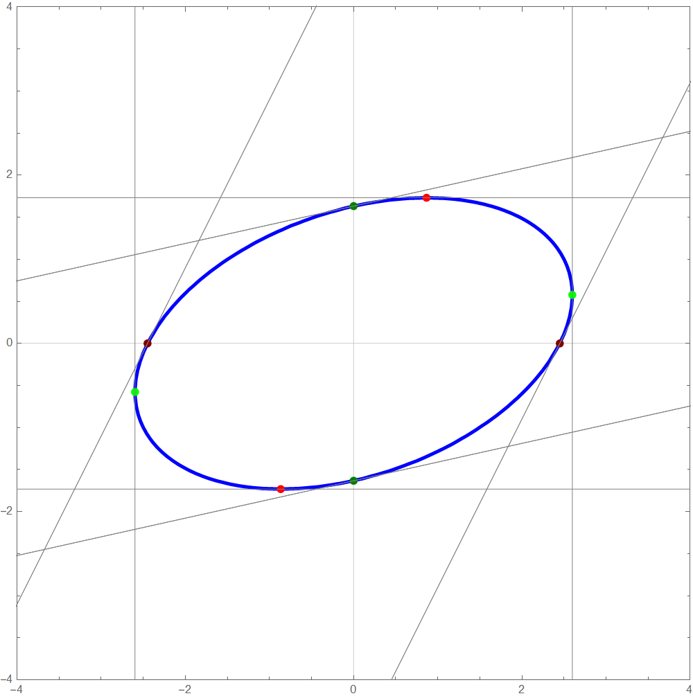
The graph of this equation in the \(xy\)-coordinate plane is an ellipse, pictured below.
- Use the implicit differentiation to find the derivatives \[ \frac{dy}{dx} \qquad \text{and} \qquad \frac{dx}{dy} \] as functions of \(x\) and \(y\).
- Calculate the \(x\)-intercepts of the given ellipse. These are the maroon points in the picture below. Recall that by definition the \(x\)-intercepts are the points which are on the ellipse and on the \(x\)-coordinate axis. Use a result obtained in item (i) to write equations of the tangent lines to the ellipse at \(x\)-intercepts.
- Calculate the \(y\)-intercepts of the given ellipse. These are the forest green points in the picture below. Recall that by definition the \(y\)-intercepts are the points which are on the ellipse and on the \(y\)-coordinate axis. Use a result obtained in item (i) to write equations of the tangent lines to the ellipse at \(y\)-intercepts.
- Use a result obtained in item (i) to calculate the points on the ellipse where the tangent lines to the ellipse are horizontal. These are the red points in the picture below.
- Use a result obtained in item (i) to find the points on the ellipse where the tangent lines to the ellipse are vertical. These are the green points in the picture below.
-
Problem. Consider the implicit equation
\[
4 x^2 - 4 x y + 9 y^2 = 24.
\]
The graph of this equation in the \(xy\)-coordinate plane is an ellipse, pictured below.
- To do the above problem it is helpful to read Example 4.30(a) in Section 4.5 Chain Rule.
-
Solution.
- To calculate \(\dfrac{dy}{dx}\) of the "function" implicitly defined by \(4 x^2 - 4 x y + 9 y^2 = 24\) we apply the chain rule to the both sides of \(4 x^2 - 4 x y + 9 y^2 = 24,\) thinking of \(y\) as a function of \(x.\) This yields \begin{align*} 0 & = \dfrac{\partial}{\partial x} \bigl( 4 x^2 - 4 x y + 9 y^2 \bigr) \dfrac{dx}{dx} + \dfrac{\partial}{\partial y} \bigl( 4 x^2 - 4 x y + 9 y^2 \bigr) \dfrac{dy}{dx} \\ & = 8x - 4 y + (-4 x + 18 y) \dfrac{dy}{dx}. \end{align*} Therefore \[ \dfrac{dy}{dx} = -\frac{8x - 4 y}{-4 x + 18 y} = \frac{4x - 2 y}{2 x - 9 y}. \] Similarly \[ \dfrac{dx}{dy} = \frac{2 x - 9 y}{4x - 2 y}. \]
- To calculate the \(x\)-intercepts of the curve \(4 x^2 - 4 x y + 9 y^2 = 24\) we substitute \(y=0\) and solve for \(x = -\sqrt{6}\) and \(x = \sqrt{6}.\) Thus, the points \(\bigl(-\sqrt{6},0\bigr)\) and \(\bigl(\sqrt{6},0\bigr)\) are the \(x\)-intercepts of the given curve. These are the maroon points in the picture. To determine the slopes of the tangent lines at these points we substitute \[ x= \sqrt{6}, \ \ y = 0 \quad \text{in} \quad \dfrac{dy}{dx} = \frac{4x - 2 y}{2 x - 9 y} \] to get that the slope is \(2.\)
- To calculate the \(y\)-intercepts of the curve \(4 x^2 - 4 x y + 9 y^2 = 24\) we substitute \(x = 0\) and solve for \(y = -2\sqrt{2/3}\) and \(y = 2\sqrt{2/3}.\) Thus, the points \(\bigl(0, -2\sqrt{2/3}\bigr)\) and \(\bigl(0, 2\sqrt{2/3}\bigr)\) are \(y\)-intercepts of the given curve. These are the forest green points in the picture. To determine the slopes of the tangent lines at these points we substitute \[ x = 0, \ \ y = 2\sqrt{2/3} \quad \text{in} \quad \dfrac{dy}{dx} = \frac{4x - 2 y}{2 x - 9 y} \] to get that the slope is \(2/9.\)
- To find the points where the tangent lines to the given curve are horizontal, we solve \[ \dfrac{dy}{dx} = \frac{4x - 2 y}{2 x - 9 y} = 0, \] giving us \(y = 2 x.\) Since we are looking for a point on the given curve, we substitute \(y=2x\) in \(4 x^2 - 4 x y + 9 y^2 = 24\) and solve for \(x.\) We obtain \[ x = - \frac{\sqrt{3}}{2}, \quad x = \frac{\sqrt{3}}{2}. \] Thus, at the points \[ \Bigl( - \frac{\sqrt{3}}{2}, - \sqrt{3} \Bigr), \quad \Bigl( \frac{\sqrt{3}}{2}, \sqrt{3} \Bigr) \] the tangent lines to the given curve are horizontal.
- To find the points where the tangent lines to the given curve are vertical, we solve \[ \dfrac{dx}{dy} = \frac{2 x - 9 y}{4x - 2 y} = 0, \] giving us \(y = (2/9) x.\) Since we are looking for a point on the given curve, we substitute \(y=(2/9) x\) in \(4 x^2 - 4 x y + 9 y^2 = 24\) and solve for \(x.\) We obtain \[ x = - \frac{3\sqrt{3}}{2}, \quad x = \frac{3\sqrt{3}}{2}. \] Thus, at the points \[ \Bigl( - \frac{3\sqrt{3}}{2}, - \frac{1}{\sqrt{3}}\Bigr), \quad \Bigl( \frac{3\sqrt{3}}{2}, \frac{1}{\sqrt{3}}\Bigr) \] the tangent lines to the given curve are vertical.
-
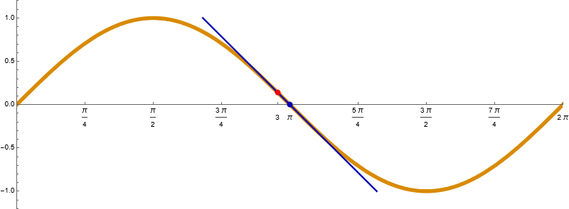
I don't think that I have recorded this problem of mine which inspired me to invent a slogan for Calculus I course:
A line is better than sine.
- Problem. Give a good rational approximation for \(\sin(3)\) using the rational approximation \(\dfrac{22}{7}\) for \(\pi.\) That is, give an approximation for \(\sin(3)\) as a fraction of two integers.
- Solution. The value of the function sine at \(\pi\) is simple \(\sin(\pi) = 0\) and the derivative is \(\sin'(\pi) = \cos(\pi) = -1.\) The tangent line to the graph of the sine function at the point \((\pi,0)\) is \[ \require{bbox} \bbox[#DDDDFF, 3px, border:3px solid #0000AA]{ y = - (x - \pi)}. \] Therefore, an approximation for \(\sin(3)\) is \[ \bbox[#DDDDFF, 3px, border:3px solid #0000AA]{ \sin(3) \approx \pi - 3}. \] To get a rational approximation for \(\sin(3)\) we are given the well-known approximation for \(\pi \approx \dfrac{22}{7}.\) Therefore \[ \sin(3) \approx \pi - 3 \approx \dfrac{22}{7} - 3 = \dfrac{1}{7}. \] Thus, \[ \sin(3) \approx \dfrac{1}{7}. \] To verify how good this approximation is, we calculate numerical approximations of \(\sin(3)\) and \(\dfrac{1}{7}\): \[ \sin(3) \approx 0.14112, \qquad \dfrac{1}{7} \approx 0.142857. \]
-
What is the analogous question for functions of two variables?
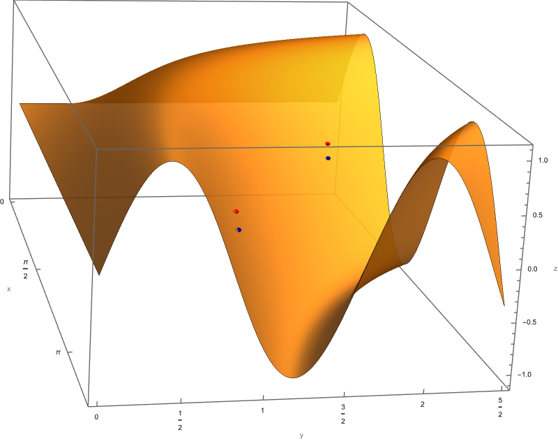
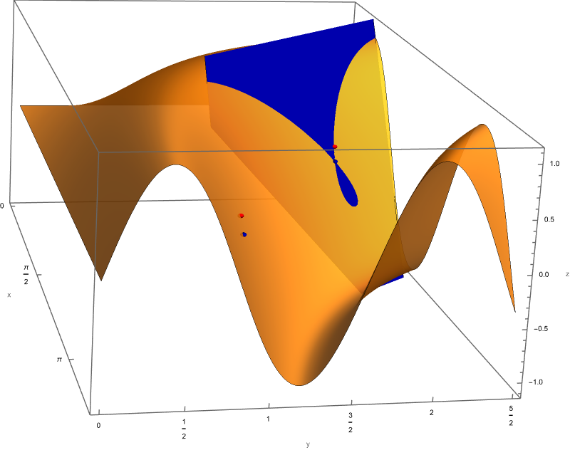
- Problem.Let \(F(x,y) = \sin(xy).\) Give a good rational approximation for the value \(F(1.5,2.01)\) using the rational approximation \(\dfrac{22}{7}\) for \(\pi.\) That is, give an approximation for \(F(1.5,2.01)\) as a fraction of two integers.
- Solution. The value of the function \(F(x,y) = \sin(xy)\) at the point \(\bbox[#DDDDFF, 3px, border:3px solid #0000AA]{(\pi/2,2)}\) is simple: \(F(\pi/2,2) = \sin(\pi) = 0.\) The point \((\pi/2,2)\) is very close to the point \(\bbox[#FFDDDD, 3px, border:3px solid #FF0000]{(1.5,2.01)}.\) Thereofre we will use the linear approximation, that is the tangent plane at the point \((\pi/2,2,0)\) to the graph of \(z=F(x,y)\) to get the rational approximation. For the tangent plane we need the partial derivatives \[ F_x(x,y) = y \cos(xy), \qquad F_y(x,y) = x \cos(xy), \] and evaluate them at the point \((\pi/2,2)\): \[ F_x(\pi/2,2) = 2 \cos(\pi) = -2, \qquad F_y(\pi/2,2) = \frac{\pi}{2} \cos(\pi) = - \frac{\pi}{2}. \] Hence, the tangent plane to the graph of \(z=F(x,y)\) at the point \((\pi/2,2,0)\) is given by \[ \require{bbox} \bbox[#DDDDFF, 3px, border:3px solid #0000AA]{ z = 0 + - 2 \Bigl(x - \frac{\pi}{2}\Bigr) - \frac{\pi}{2} (y - 2) }. \] Therefore, an approximation for \(F(1.5,2.01)\) is \[ \bbox[#DDDDFF, 3px, border:3px solid #0000AA]{ F(1.5,2.01) \approx - 2 \Bigl(\frac{3}{2} - \frac{\pi}{2}\Bigr) - \frac{\pi}{2} (2.01 - 2) = \pi - 3 - \frac{\pi}{200} }. \] To get a rational approximation for \(F(1.5,2.01)\) we are given the well-known approximation for \(\pi \approx \dfrac{22}{7}.\) Therefore \[ F(1.5,2.01) \approx \pi - 3 - \frac{\pi}{200} \approx \dfrac{22}{7} - 3 - \dfrac{\dfrac{22}{7}}{200} = \dfrac{1}{7} - \dfrac{11}{700} = \dfrac{89}{700}. \] Thus, \[ F(1.5,2.01) \approx \dfrac{89}{700}. \] To verify how good this approximation is, we calculate numerical approximations of \(F(1.5,2.01)\) and \(\dfrac{89}{700}\): \[ F(1.5,2.01) \approx 0.126255, \qquad \dfrac{89}{700} \approx 0.126801. \]
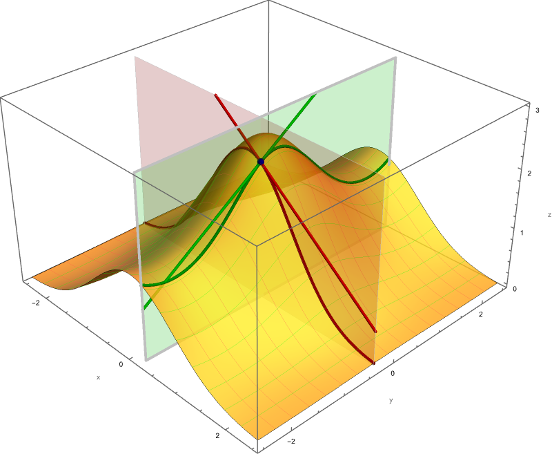
- The picture below shows the graph of \(z=F(x,y)\) together with its blue tangent plane at the point \((\pi/2,2,0).\)
-
To get the rational approximation in the preceding problem we used the tangent plane approximation of the surface that looks like a wave. Therefore, a slogan for this class
A plane is better than a wave.
-
This is a part of Section 4.4 Tangent Planes and Linear Approximations in OpenStax Calculus Volume 3. More linear approximation problems you can find among the problems in this sections: 163, 169, 170, 181, 182, 183, 187, 188, 189, 190, 194, 195, 207, 208, 211.
- Below is an illustration of a vibrating string. Its equation is $y = u(x,t) = (\sin x) (\cos t)$.The Partial differential equation governing the vibrations of this string is \[ \frac{\partial^2 u}{\partial t^2}(x,t) = \frac{\partial^2 u}{\partial x^2}(x,t) \quad \text{where} \quad 0 \leq x \leq \pi, \quad t \geq 0 \] In the figure below $y$ is the vertical axis, $x$ is the horizontal axis and the time $t$ is displayed above the frame. The string at time $t$ is black. To indicate the motion of the string, I added several previous positions of the string in various shade of gray. In fact, the previous positions fade away. At each point in time $t_0 \in [0, 2 \pi)$ and for each point $x_0 \in [0,\pi]$ you should be able to determine the sign of the following quantities: \begin{align*} & u(x_0,t_0), \\ & u_x(x_0,t_0), \ \ u_t(x_0,t_0), \\ & u_{xx}(x_0,t_0), \ \ u_{xt}(x_0,t_0), \ \ u_{tx}(x_0,t_0), \ \ u_{tt}(x_0,t_0). \end{align*} The best way to achieve this is to understand the meaning of each of these quantities. In fact, you should be able to determine the signs of the quantities listed above just based on one scene in the movie below and just based on a point emphasized on the graph of the string (even without explicitly given the values for $x_0$ and $t_0$).
-
Today we finished by starting Section 4.4 Tangent Planes and Linear Approximations in OpenStax Calculus Volume 3. Do as many problems from 163 to 214 as you can. In particular: 163, 169, 170, 181, 182, 183, 187, 188, 189, 190, 194, 195, 207, 208, 211.
-
The following three pictures illustrate how we calculate the tangent plane from the partial derivatives.


Clicking on the image will cycle through 8 different individual scenes of this movie with various values of $x_0 \in [0,\pi]$.
-
Today we started Section 4.3 Partial Derivatives in OpenStax Calculus Volume 3. Do as many problems from 112 to 162 as you can. In particular: 112, 115, 116, 117, 118, 119, 122, 127, 129, 137, 138, 139, 141, 145, 148, 149, 152, 153, 158, 159.
-
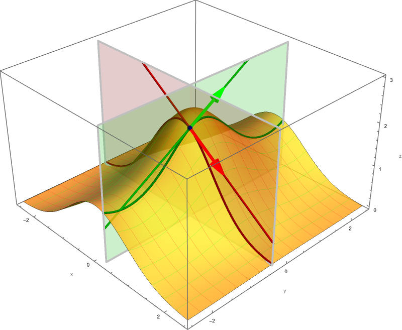
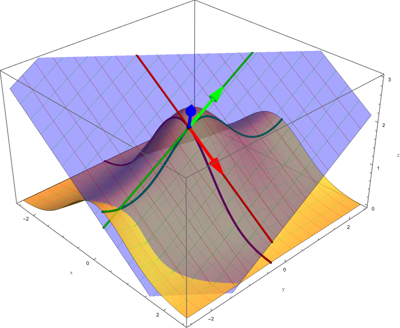
Below is a canonical color-coded illustration of the partial derivative at a navy blue point. All shades of red relate to the partial derivative with respect to \(x,\) and all shades of green relate to the partial derivative with respect to \(y.\)
-
In Section 4.2, Limits and Continuity, the book presents the \(\require{ams}\epsilon\text{-}\delta\) definitions of limit and continuity. I regard these \(\epsilon\text{-}\delta\) definitions as one of humanity’s highest intellectual achievements. We tried to convey their spirit within the short time we devoted to this topic.
Here is a link to a song celebrating \(\epsilon\text{-}\delta\) definitions, Lyrics: Tom Lehrer — “There’s a Delta for Every Epsilon” or Tom Lehrer at YouTube
-
Today we started Section 4.2 Limits and Continuity in OpenStax Calculus Volume 3.
-
In this section we study limits of the form \[ \lim_{(x,y)\to (a,b)} f(x,y). \] Here \(f\) is a function of two variables with real numbers as values.
In all examples in this section, the function \(f(x,y)\) is given by an algebraic formula, that is, a formula built from constants, variables, and the operations of addition, subtraction, multiplication, division, and taking roots, or familiar exponential function, logarithms, or trigonometric functions.
There are two distinct cases:
-
The point \((a,b)\) is in the domain of the function \(f(x,y)\), that is we can evaluate the value \(f(a,b).\) In this case we have \[ \lim_{(x,y)\to (a,b)} f(x,y) = f(a,b). \] That is, functions given by algebraic formulas are continuous wherever they are defined. Thus, to find the limit of such a function at a point in its domain, you can simply substitute the point into the formula.
Example 4.8 and Exercises 60, 61, 63, 64, 66-75 all belong to this kind of problems.
-
The point \((a,b)\) is NOT in the domain of the function \(f(x,y)\), that is, the value \(f(a,b)\) is not defined. A limit \[ \lim_{(x,y)\to (a,b)} f(x,y) \] of this kind is more difficult to asses. In some examples the limit exists, and we have to figure out what it is and make the argument why that limit is what we claim it is. Sometimes the limit simply does not exist and we provide argument why.
Example 4.9 explains how to deal with limits of this kind. Exercises 86, 87, 88, 89 are similar. Exercises 65, 76, 77, 80, 81, 82, 83 belong to this kind of problems, some of these limits exist, some do not.
Three examples of limits of this kind that do exist are as follows: \[ \lim_{(x,y)\to (0,0)} \frac{x y }{|x| + |y|} = 0, \] \[ \lim_{(x,y)\to (0,0)} \frac{x^2 y }{x^2 + y^2} = 0, \] \[ \lim_{(x,y)\to (0,0)} \frac{x y }{\sqrt{x^2 + y^2}} = 0. \] And three that do not exist \[ \lim_{(x,y)\to (0,0)} \frac{x + y }{|x| + |y|}, \] \[ \lim_{(x,y)\to (0,0)} \frac{x y}{x^2 + y^2}, \] \[ \lim_{(x,y)\to (0,0)} \frac{x + y }{\sqrt{x^2 + y^2}}. \]
-
- Today we did Section 4.1 Functions of Several Variables in OpenStax Calculus Volume 3. Do as many problems as you can from 1 to 59. In particular: 2, 3, 5, 6, 8, 9, 11, 12, 13-20, 30, 32, 33, 36, 39, 40, 42, 43, 44, 45, 46, 47, 48, 49, 50, 51, 53.
-
Here I present animations of cross sections of a graph of $z = y^2-x^2$ by planes parallel to $xy$-plane, $zx$-plane and $yz$-plane, respectively.
Place the cursor over an image to start the animation.
-
Here I present animations of cross sections of a little bit more interesting graph of $z = y^3 + xy.$ As above, the cross sections are by planes parallel to $xy$-plane, $zx$-plane and $yz$-plane, respectively.
Place the cursor over an image to start the animation.
-
All illustrations on my website are produced with Wolfram Mathematica. Mathematica is a tool for doing mathematics on the computer. You can think of it as a super-powerful graphing calculator. It can do symbolic and numerical calculations, produce simple and sophisticated graphics, all in one environment.
You will definitely benefit from taking some interest in it. To get started with Mathematica, visit my Mathematica page. It contains links to several videos that will help you get started efficiently. Mathematica is available in the computer labs in BH 215, CF 312, HH 233, and BH 209.
Below is Wolfram Mathematica code to plot the function \(f(x,y) = y^3 + x y\).
Plot3D[y^3 + x y, {x, -3.5, 2.5}, {y, -2.5, 2.5},
 PlotRange -> {{-3.5, 2.5}, {-2.5, 2.5}, {-4, 4}},
 PlotPoints -> {201, 201}, PlotStyle -> Directive[Opacity[0.6]],
 Mesh -> True, AxesLabel -> {"x", "y", "z"}, BoxRatios -> {1, 1, 1},
 ClippingStyle -> None, ImageSize -> 600]
Below is Wolfram Mathematica code to plot the function \(f(x,y) = \sqrt{4 - x^2 - y^2}\).
Plot3D[Sqrt[4 - x^2 - y^2], {x, -2.5, 2.5}, {y, -2.5, 2.5},
 PlotRange -> {{-2.5, 2.5}, {-2.5, 2.5}, {0, 3}},
 PlotPoints -> {201, 201}, PlotStyle -> Directive[Opacity[0.8]],
 Mesh -> True, AxesLabel -> {"x", "y", "z"}, BoxRatios -> {5, 5, 3},
 ClippingStyle -> None, ImageSize -> 600]
You can copy and paste the above code directly into a Mathematica notebook. Then press , and Mathematica will display a plot of the function. You can modify the code to adjust the plot to your liking.
Large Language Models are very good at giving advice on how to do things in Wolfram Mathematica. I have used ChatGPT, Gemini, Copilot, and DeepSeek, and have had both extremely positive and negative experiences with each of them. Overall, the experience has been overwhelmingly positive. Using LLMs to improve your computer skills is a great way to learn through interaction. When you ask an LLM to provide code for a task, it is usually easy to assess whether the code works. If you try different LLMs for the same task, you may be surprised by how different their answers can be.
- Our next topic is Section 4.1 Functions of Several Variables in OpenStax Calculus Volume 3. Do as many problems as you can from 1 to 59. In particular: 2, 3, 5, 6, 8, 9, 11, 12, 13-20, 30, 32, 33, 36, 39, 40, 42, 43, 44, 45, 46, 47, 48, 49, 50, 51, 53.
-
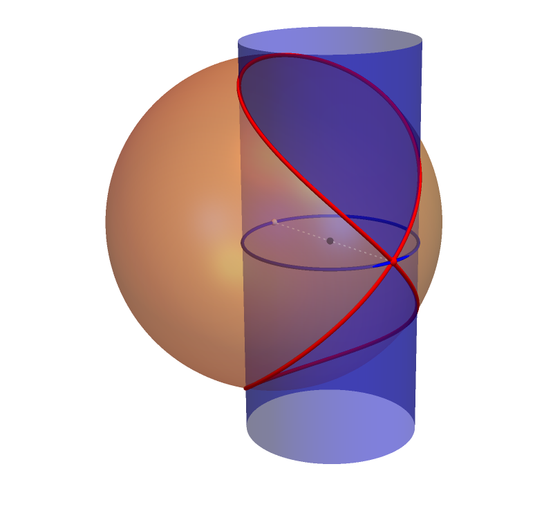
Before moving on to the new topic, I wanted to share with you the derivation of the parametric equations of the Viviani Curve, Problem 355 in Section 2.6. The Viviani Curve is the intersection of the sphere of radius \(2\) centered at the origin and the circular cylinder or radius \(1\) whose axis is the line \(x=1, y = 0, z = t\) where \(t \in \mathbb{R}.\)
In set notation the Viviani Curve is the following intersection \[ \Bigl\{ (x,y,z ) \in \mathbb{R}^3 \ \bigl| \bigr. \ x^2 + y^2 + z^2 = 4 \Bigr\} \, \bigcap \,\Bigl\{ (x,y,z) \in \mathbb{R}^3 \ \bigl| \bigr. \ (x-1)^2 + y^2 = 1 \Bigr\}. \]
I vividly remember being assigned the Viviani Curve in my calculus class in 1975 at the University of Sarajevo. Now, half a century later, this animation is my tribute to that beautiful mathematical concept.
The animation below illustrates how the curve's parametrization is obtained. To help you follow along, the light gray dashed lines represent vectors, and the white point is the origin.
The constant vector is \(\mathbf{i}\). The vector that is added to \(\mathbf{i}\) is the vector \[ (\cos \theta) \mathbf{i} + (\sin \theta) \mathbf{j}. \] Here, \(\theta\) can be any real number, although, later on we will realize that it is sufficient to take \(\theta\) such that \(0 \leq \theta \leq 4 \pi.\) Why are these two vectors important? When added together, we get \[ \mathbf{i} + (\cos \theta) \mathbf{i} + (\sin \theta) \mathbf{j} = \bigl(1+ \cos \theta \bigr) \mathbf{i} + (\sin \theta) \mathbf{j}. \] The head of this vector, the point \[ \bigl( 1+ \cos \theta, \sin \theta, 0 \bigr) \] is on the cylinder \[ \Bigl\{ (x,y,z) \in \mathbb{R}^3 \ \bigl| \bigr. \ (x-1)^2 + y^2 = 1 \Bigr\}. \] In fact, for any \(z \in \mathbb{R}\), the point \[ \bigl( 1+ \cos \theta, \sin \theta, z \bigr) \] is on that cylinder. Therefore, we just need to find \(z\) for which the point \[ \bigl( 1+ \cos \theta, \sin \theta, z \bigr) \] is on the sphere \[ \Bigl\{ (x,y,z ) \in \mathbb{R}^3 \ \bigl| \bigr. \ x^2 + y^2 + z^2 = 4 \Bigr\}. \] To calculate such \(z\) we substitute the point \[ \bigl( 1+ \cos \theta, \sin \theta, z \bigr) \] into \[ x^2 + y^2 + z^2 = 4 \] and solve for \(z\): \[ (1+ \cos \theta)^2 + (\sin\theta)^2 + z^2 = 4. \] Simplifying the last expression yields \[ z^2 = 2(1 - \cos\theta). \] As often, trigonometric identities are useful whenever we encounter trigonometric functions. Here, the half-angle formula for \(\cos\theta\) does the magic: \[ \cos\theta = \cos^2\Bigl(\frac{\theta}{2}\Bigr) - \sin^2\Bigl(\frac{\theta}{2}\Bigr) \] and \[ 1 = \cos^2\Bigl(\frac{\theta}{2}\Bigr) + \sin^2\Bigl(\frac{\theta}{2}\Bigr). \] Therefore, \[ 1 - \cos\theta = 2 \sin^2\Bigl(\frac{\theta}{2}\Bigr). \] Hence \[ z^2 = 4 \sin^2\Bigl(\frac{\theta}{2}\Bigr). \] It turns out that all the solutions for \(z\) are given by \[ z = 2 \sin\Bigl(\frac{\theta}{2}\Bigr) \quad \text{where} \quad 0 \leq \theta \leq 4 \pi. \] Thus the vertical dashed vector is \[ 2 \sin\Bigl(\frac{\theta}{2}\Bigr) \, \mathbf{k}. \] This vector starts at the blue dot on the blue circle and ends at the sphere.
This is how to reach a point on the Viviani Curve from the origin \[ \underbrace{\mathbf{i}}_{\text{the first dashed vector}} + \underbrace{(\cos \theta) \mathbf{i} + (\sin \theta) \mathbf{j}}_{\text{the second dashed vector}} + \underbrace{2 \sin\Bigl(\frac{\theta}{2}\Bigr) \, \mathbf{k}}_{\text{the third dashed vector}}. \]
Thus the parametric equations of the Viviani Curve are \[ x = 1 + \cos\theta, \quad y = \sin\theta, \quad z = 2 \sin\Bigl(\frac{\theta}{2}\Bigr), \quad \text{where} \quad 0 \leq \theta \leq 4 \pi. \]
Let us verify that these points are on the sphere. It is convenient to rewrite the parametric equations using the half-angle formulas again: \[ x = 2 \Bigl(\cos \frac{\theta}{2}\Bigr)^2, \quad y = 2\Bigl( \sin \frac{\theta}{2}\Bigr) \Bigl(\cos \frac{\theta}{2}\Bigr), \quad z = 2 \sin\Bigl(\frac{\theta}{2}\Bigr), \quad \text{where} \quad 0 \leq \theta \leq 4 \pi. \] Then \begin{align*} x^2 + y^2 + z^2 & = 4 \Bigl( \cos \frac{\theta}{2} \Bigr)^4 + 4 \Bigl( \sin \frac{\theta}{2} \Bigr)^2 \Bigl( \cos \frac{\theta}{2} \Bigr)^2 + 4 \Bigl(\sin \frac{\theta}{2} \Bigr)^2 \\ & = 4 \Bigl( \cos \frac{\theta}{2} \Bigr)^2 \biggl( \Bigl( \cos \frac{\theta}{2} \Bigr)^2 + \Bigl( \sin \frac{\theta}{2} \Bigr)^2 \biggr) + 4 \Bigl(\sin \frac{\theta}{2} \Bigr)^2 \\ & = 4 \Bigl( \cos \frac{\theta}{2} \Bigr)^2 + 4 \Bigl(\sin \frac{\theta}{2} \Bigr)^2 \\ & = 4. \end{align*}
Place the cursor over the image to start the animation.
- This webpage, was linked in Canvas discussions since it somewhat indicates how vectors are used in navigation. In the middle of the page it also mentions that certain distortions occur on the so-called "limacon pattern" (cardioid) pattern. Inspired by this, below I deduce parametric equations for a cardioid and a limacon.
-
The following table presents a derivation of the equation of a cardioid. For optimal viewing, use a wide screen.
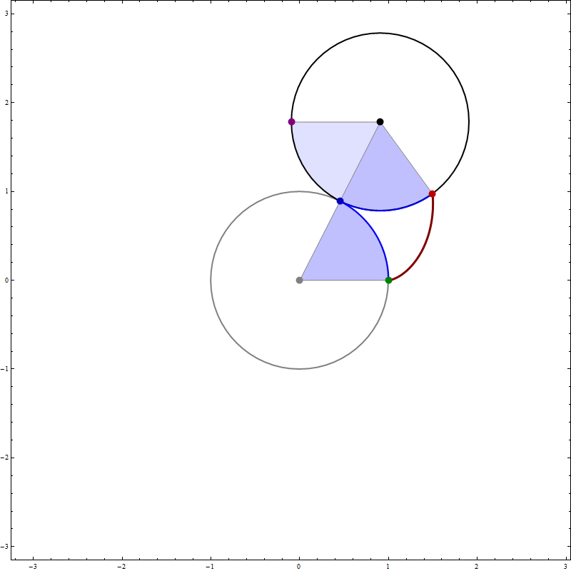
Click through several helpful images.
- The origin $O = (0,0)$ of the coordinate system is the gray point. Denote by $C$ the black point in the picture.
- Both circles in the picture are unit circles, the gray one centered at $O,$ the black one centered at $C.$
- The angle at the gray point marked by the blue arc between the green and the blue point measures $t$ radians. That is, the length of this blue arc is $t.$
- There are two other angles in the picture which also measure $t$ radians: the angle marked by the blue arc between the blue and the red point and the angle marked by the black arc between the blue point and the purple point.
- The green point is $(1,0),$ the blue point is $(\cos t, \sin t),$ the black point $C$ is $(2\cos t, 2\sin t),$ the purple point is $(2\cos t-1, 2\sin t).$
- The goal is to determine the coordinates of the red point.
- Denote by $\mathbf{a}$ the unit vector whose tail is the black point and whose head is the red point. Based on the previous items we have \begin{align*} \mathbf{a} & = \bigl(\cos( \pi+2 t ) \bigr) \mathbf{i} + \bigl(\sin( \pi+2 t ) \bigr) \mathbf{j} \\ & = -\bigl(\cos(2 t ) \bigr) \mathbf{i} - \bigl(\sin(2 t ) \bigr) \mathbf{j}. \end{align*}
- Denote by $\mathbf{c}$ the position vector of the black point. Then the position vector of the red point is \[ \mathbf{c} + \mathbf{a} = \bigl( 2 \cos t - \cos(2 t ) \bigr) \mathbf{i} + \bigl(2 \sin t - \sin(2 t ) \bigr) \mathbf{j}. \]
- Thus the parametric equations for this cardioid are \begin{align*} x & = 2 \cos t - \cos(2 t ) \\ y & = 2 \sin t - \sin(2 t ) \end{align*}
-
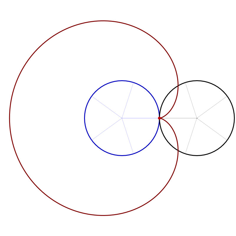
This is Cardioid similar to the one on Wikipidia's Cardioid page
Place the cursor over the image to start the animation.
-
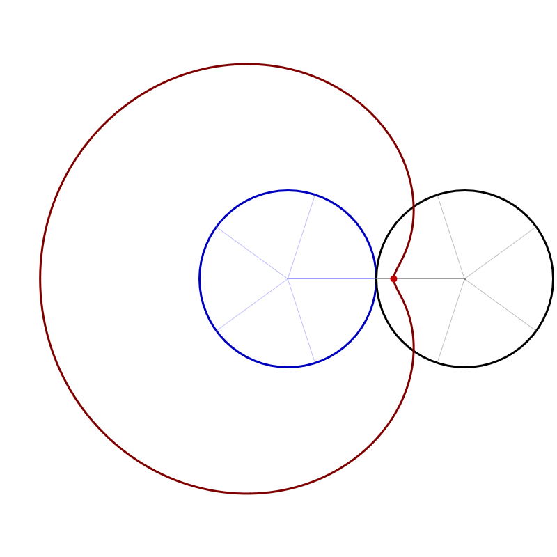
This is a Limaçon similar to the one on Wikipidia's Limaçon
Place the cursor over the image to start the animation.
-
There was a question in class today about the notation \(\cos^{-1}\) in relation to \(\arccos\). My answer was that the notation \(\cos^{-1}\) is wrong. I will explain my reasoning below.
-
Let \(f\) be a function. What does \(f^{-1}\) mean? We can consult Wikipedia Inverse function; we find
-
The key sentence is:
The inverse of \(f\) exists if and only if \(f\) is bijective, and if it exists, is denoted by \(\displaystyle f^{-1}.\)To my taste, the highlighted sentence is too terse. I would prefer to restate it as follows:
The inverse of \(f\) exists if and only if \(f\) is bijective. If \(f\) is bijective, that is if the inverse of \(f\) exists, then the inverse of \(f\) is denoted by \(\displaystyle f^{-1}.\)
Now, I see that some might complain that my highlighted paragraph above is somewhat repetitive; I phrase it so to be absolutely clear, and to emphasise the following important implication
If the inverse of \(f\) exists, then the inverse of \(f\) is denoted by \(\displaystyle f^{-1}.\) -
From the preceding item, to understand the inverse of a function \(f\) we must understand what it means for a function \(f\) to be bijective. Again, Wikipedia is helpful, Bijection. Please read carefully the definition below.
A bijection, or bijective function is a function between two sets such that each element of the second set (the codomain) is the image of exactly one element of the first set (the domain). Equivalently, a bijection is a relation between two sets such that each element of either set is paired with exactly one element of the other set.Now we go back to the concept of an inverse function
Or, briefly,The inverse of \(f\) exists if and only if \(f\) is bijective. If \(f\) is bijective, that is if the inverse of \(f\) exists, then it is denoted by \(\displaystyle f^{-1}.\)If \(f\) is bijective, then the inverse of \(f\) is denoted by \(\displaystyle f^{-1}.\) - In conclusion, in order to talk about \(f^{-1}\) we need to establish that the function \(f\) is bijective. Thus, to use \(\cos^{-1}\) we would need to establish that the function \(\cos\) is a bijection. The most common understanding of this function is that its domain is the set \(\mathbb{R}\) and its range is the closed interval \([-1,1].\) With this domain and the function cosine is NOT a bijection. I can restrict it domain to the closed interval \([0,\pi],\) but then that is not the same function. So, I can define a new function \[ \operatorname{mycos}: [0,\pi] \to [-1,1], \quad \operatorname{mycos}(x) = \cos(x) \quad \text{for all} \quad x \in [0,\pi]. \] The function \(\operatorname{mycos}\) is a bijection. Therefore, I can use \(\operatorname{mycos}^{-1}.\) In fact, this is exactly how the function \(\arccos\) is defined: \(\arccos\) is the inverse function of the bijection \(\operatorname{mycos}\).
-
Let \(f\) be a function. What does \(f^{-1}\) mean? We can consult Wikipedia Inverse function; we find
- To help clarify some common questions about functions, I wrote the Functions webpage.
- We started Section 2.6 Quadric Surfaces in OpenStax Calculus Volume 3.
-
It is essential to understand the shape of surfaces with one of the following three kinds of equations:
-
\( a x^2 + b y^2 + c z^2 = d, \) where \(a, b, c, d\) are any of the numbers \(-1,0,1.\) For example, \[ x^2 + y^2 - z^2 = 1, \quad x^2 + y^2 - z^2 = 0, \quad x^2 + y^2 - z^2 = -1, \] or \[ x^2 - y^2 + z^2 = 1, \quad x^2 - y^2 + z^2 = 0, \quad x^2 - y^2 + z^2 = -1. \]
-
$ a x^2 + b y^2 + c z = d, $ where \(a, b, c, d\) are any of the numbers \(-1,0,1.\) For example, \[ z = x^2 + y^2, \quad z = x^2 - y^2, \quad z = x^2, \quad z = y^2, \] or, \[ x^2 + y^2 = 1, \quad x^2 - y^2 = 1, \quad x^2 = y^2. \]
-
$ a x^2 + b y + c z^2 = d, $ where \(a, b, c, d\) are any of the numbers \(-1,0,1.\) For example, \[ y = x^2 + z^2, \quad y = x^2 - z^2, \quad y = x^2, \quad y = z^2, \] or, \[ x^2 + z^2 = 1, \quad x^2 - z^2 = 1, \quad x^2 = z^2. \]
-
$ a x + b y^2 + c z^2 = d, $ where \(a, b, c, d\) are any of the numbers \(-1,0,1.\) For example, \[ x = y^2 + z^2, \quad x = y^2 - z^2, \quad x = y^2, \quad x = z^2, \] or, \[ y^2 + z^2 = 1, \quad y^2 - z^2 = 1, \quad y^2 = z^2. \]
-
-
Since my focus here is different from the focus in the book, the homework from the OpenStax is limited:
- Look at graphs in Problems 309, 310, 311, and 312. Find a possible equation for each graph among the equations presented in the preceding item.
- For Problems 313, 314, 315, 316, 317, 318, six formulas are given in a, b , c, d, e, f. Replace these equations with \begin{alignat*}{3} x^{2} + y^{2} - z^{2} & = 1, & \quad x^{2} - y^{2} - z^{2} & = 1, & \quad x^{2} + y^{2} + z^{2} & = 1, \\ x^{2} + y^{2} - z & = 0, & \quad x^{2} - y^{2} - z & = 0, & \quad x^{2}+y^{2}-z^{2} & = 0. \end{alignat*} And replace the surface names with: Hyperboloid of two sheets, Sphere, Paraboloid, Hyperbolic paraboloid, Hyperboloid of one sheet, Cone.
- Problem 338 is interesting.
-
Problem 355 is exceptionally interesting. I remember being assigned exactly the same problem when I was an undergraduate student. This is not something that can appear on exam. It is an interesting exercise in obtaining parametric equations of the Viviani curve:
\[
x(t) = 1 + \cos(t), \quad y(t) = \sin(t), \quad z(t) = 2 \sin(t/2), \quad -2 \pi \leq t \leq 2 \pi.
\]
-
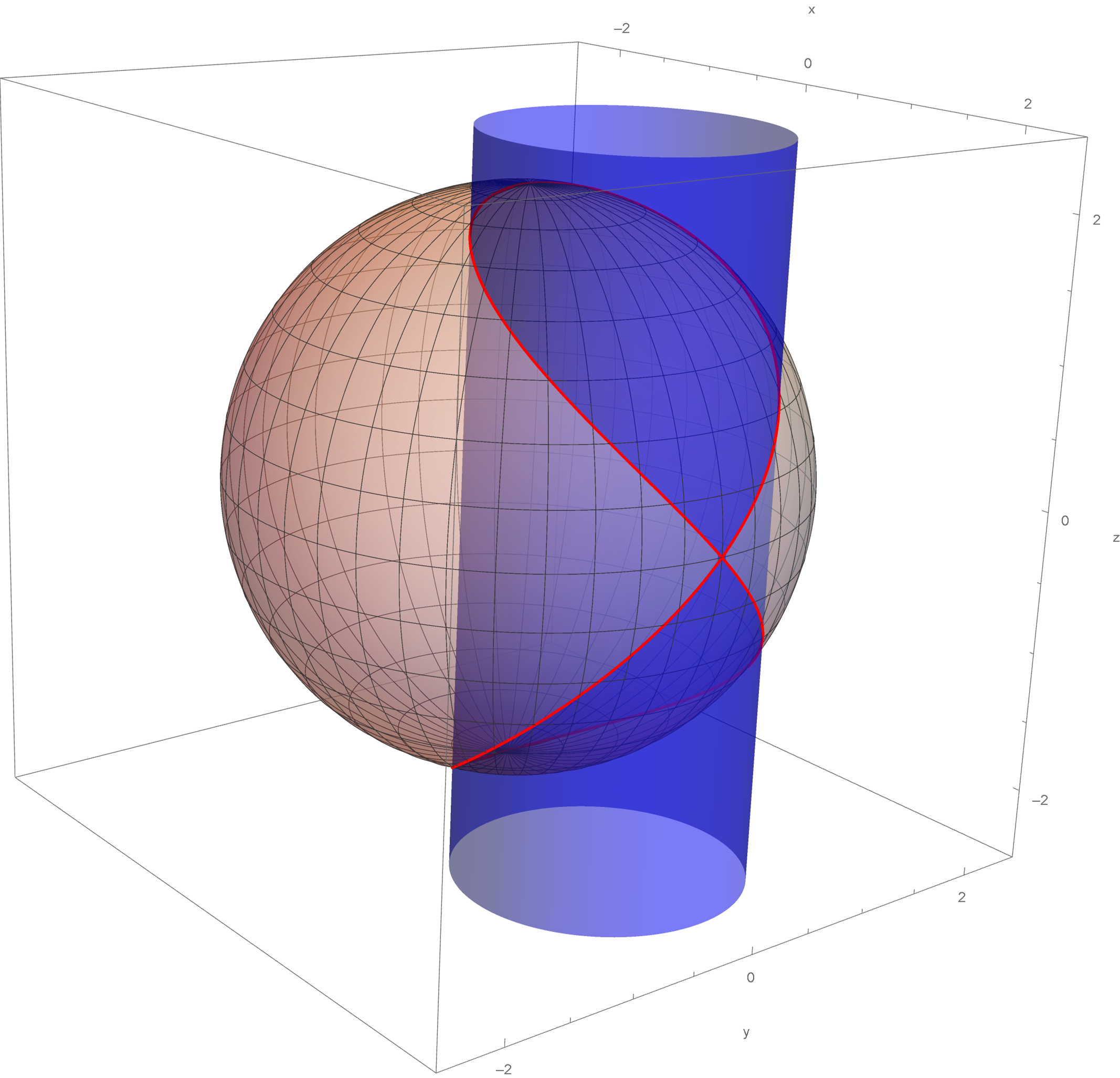
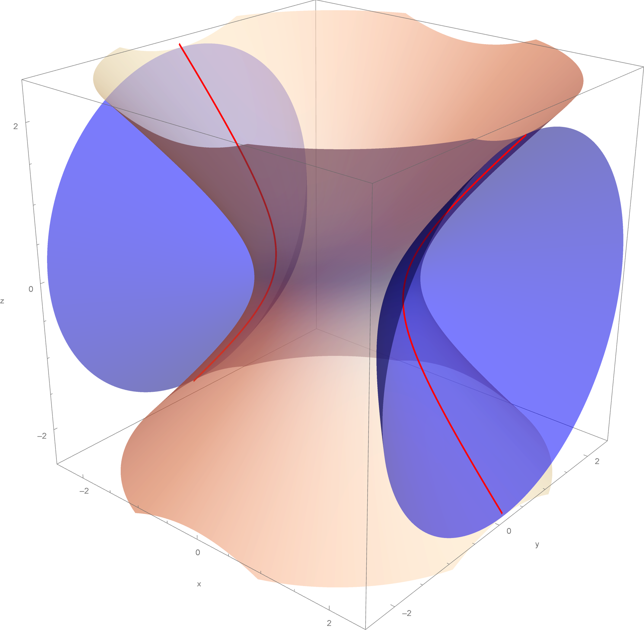
Problem 356 is also interesting. Although, the picture provided looks inaccurate. The second surface is a cone and its vertex is at the origin. The provided picture does not show the vertex at the origin. But, I am not interested in these complicated equations. I would look at a simple hyperboloid and a simple cone: \[ x^2 + y^2 - z^2 = 1, \qquad -x^2 + y^2 + z^2 = 0. \] Substituting \(x^2 = y^2 + z^2\) from the second equation, into the first, we get \(2 y^2 = 1\). Hence, the intersection of these two surfaces lies in two planes parallel to \(xz\)-coordinate plane. One such plane is \(y =\sqrt{2}/2\) and the other is \(y = -\sqrt{2}/2.\) Thus, the intersection is given by the equations: \[ x^2 - z^2 = 1/2, \qquad y^2 = 1/2. \]
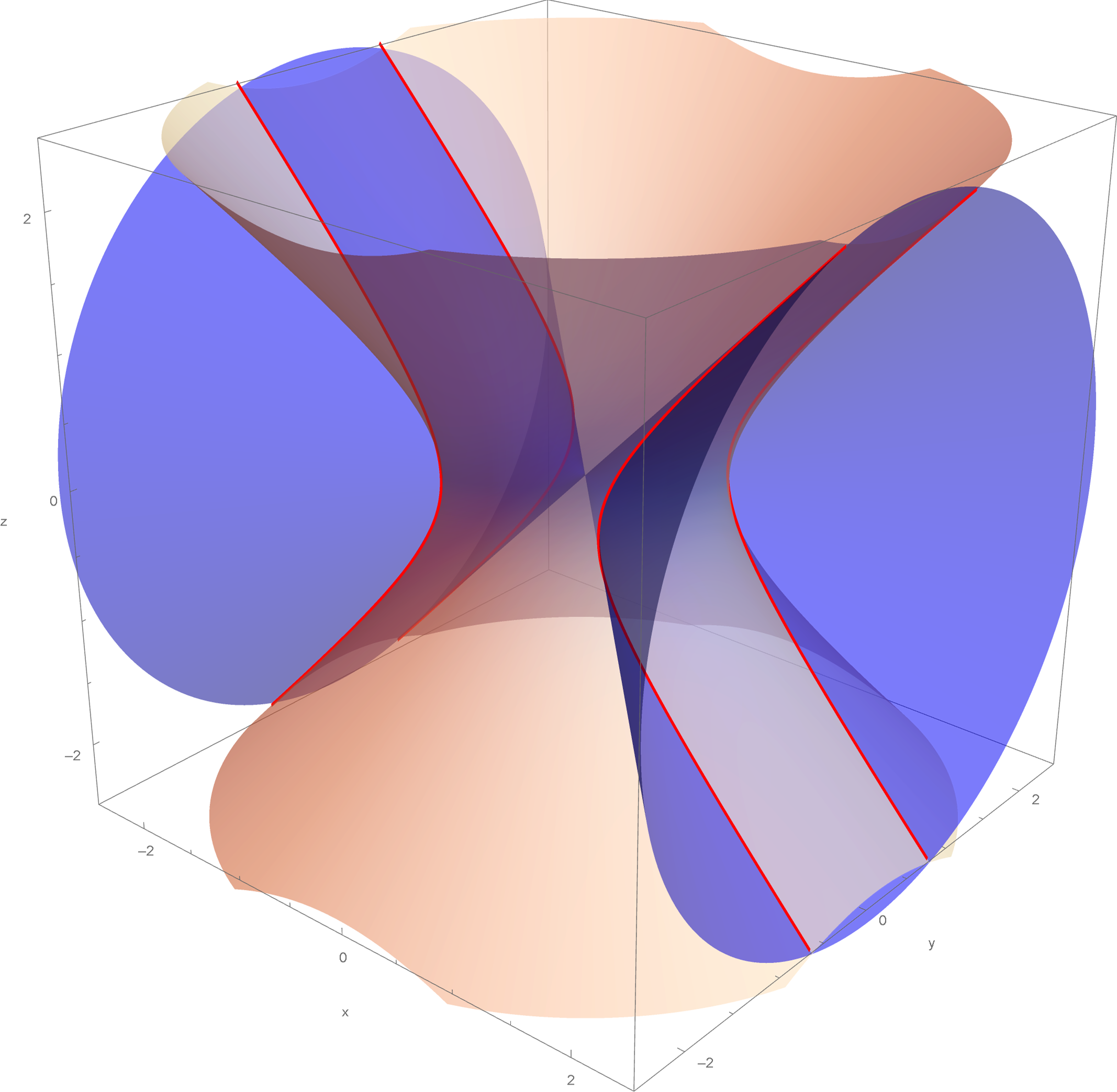
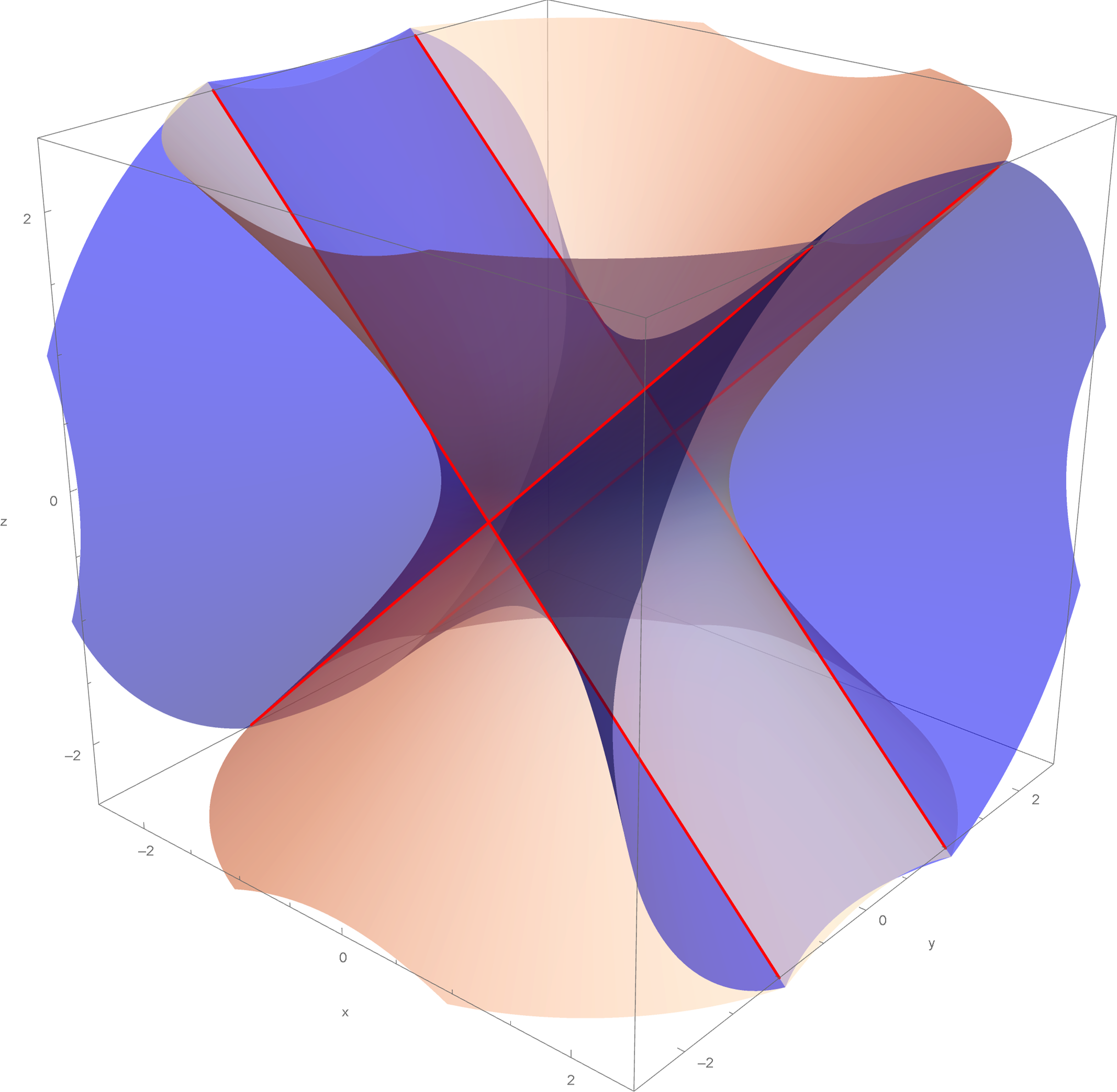
We can replace cone in Problem 356 with a horizontal hyperboloid of one sheet and consider the intersection of the surfaces \[ x^2 + y^2 - z^2 = 1, \qquad -x^2 + y^2 + z^2 = 1. \] Substituting \(x^2 = y^2 + z^2 - 1\) from the second equation into the first, we get \(2 y^2 = 2\). Hence, the intersection of these two surfaces lies in two planes parallel to \(xz\)-coordinate plane. One such plane is \(y = 1\) and the other is \(y = -1.\) Thus, the intersection is given by the equations: \[ x^2 - z^2 = 0, \qquad y^2 = 1. \]
Finally, we can replace cone in Problem 356 with a horizontal hyperboloid of two sheets and consider the intersection of the surfaces \[ x^2 + y^2 - z^2 = 1, \qquad -x^2 + y^2 + z^2 = -1. \] Substituting \(x^2 = y^2 + z^2 + 1\) from the second equation into the first, we get \(2 y^2 = 0\). Hence, the intersection of these two surfaces lies in the \(xz\)-coordinate plane. Thus, the intersection is given by the equations: \[ x^2 - z^2 = 1, \qquad y = 0. \]
-
Hyperboloids are present in art and architecture. Below is an animation that might help you understand the shape of the surface with the equation $x^2 + y^2 - z^2 = c$ for different values of $c$. You can read more at the Wikipedia
Hyperboloid page. One sheet hyperboloids are often encountered in art, see these Wikipedia pages Hyperboloid structure and list of hyperboloid structures, do not miss the Gallery at the bottom of the last Wikipedia page.
Place the cursor over the image to start the animation.
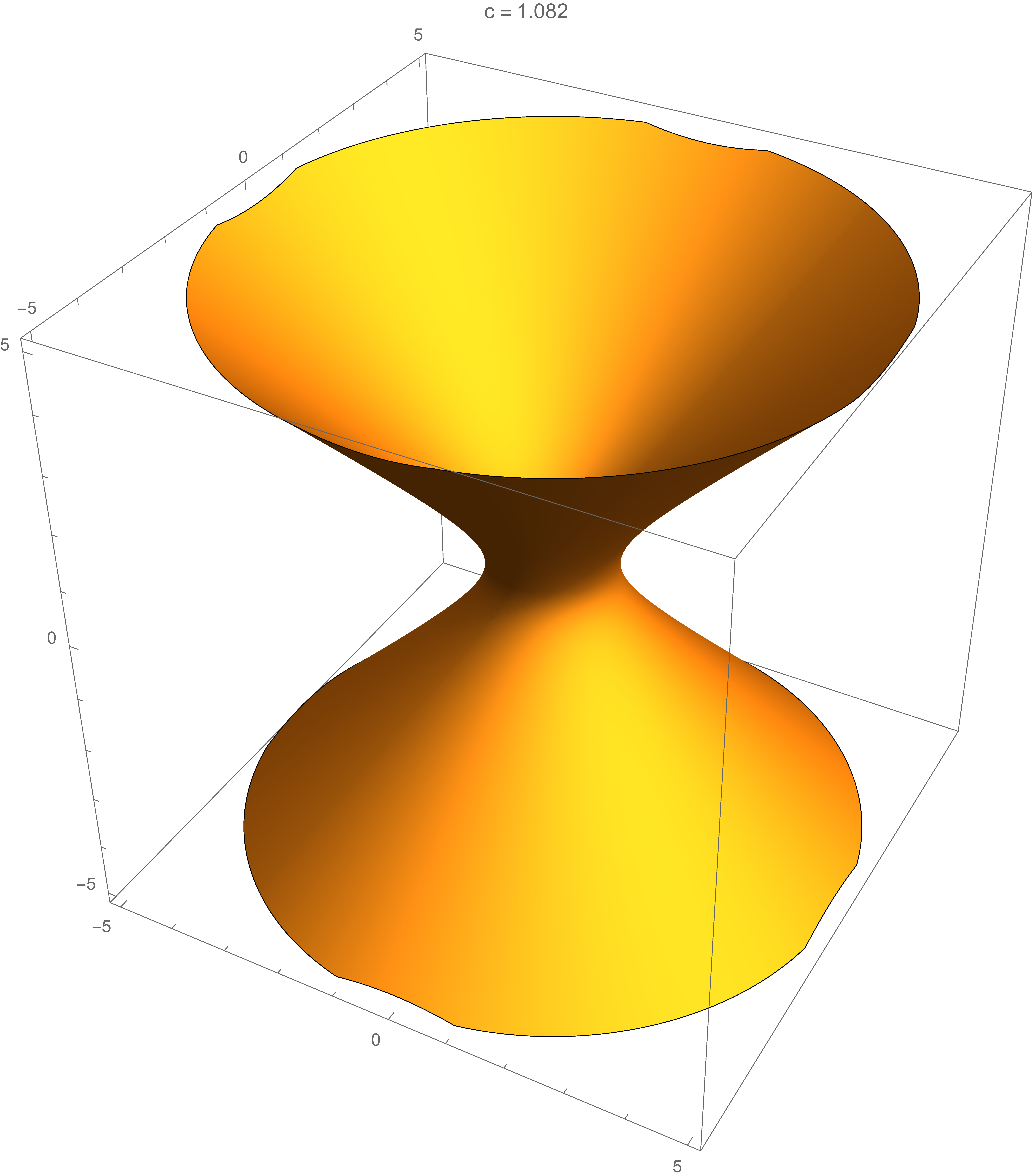
Five of the above level surfaces at different level of opacity.

- Today we talked about the the scalar triple product of three vectors \(\mathbf{a}\), \(\mathbf{b}\), and \(\mathbf{c}\), that is \[ (\mathbf{a}\times \mathbf{b})\cdot \mathbf{c}. \] The absolute value of this product is the volume of the parallelepiped formed by \(\mathbf{a}\), \(\mathbf{b}\), and \(\mathbf{c}\). See yesterday post for more details.
-
My favorite application of vectors: COLORS. In fact, I love this application so much that I wrote a webpage to celebrate it: Color Cube.
One exercise in this context would be to ask you to find three colors which are between teal and yellow, one in the middle between teal and yellow and the other two in the middle between teal and the mid-color and in the middle of mid-color and yellow.
- We started Section 2.5 Equations of Lines and Planes in Space in OpenStax Calculus Volume 3. Do as many problems as you can from 243 to 302. In particular: 243, 244, 248, 250, 251, 254, 255, 257, 259, 263, 266, 268, 272, 275, 279, 280, 282, 285, 287, 289, 290, 292, 293, 295, 298.
-
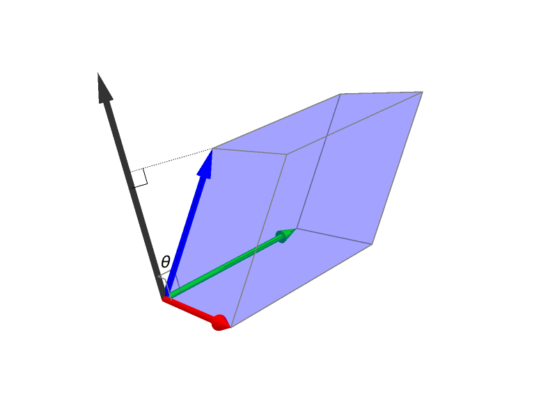
In the picture below, the red vector is \(\mathbf{a}\), the green vector is \(\mathbf{b}\), and the blue vector is \(\mathbf{c}.\) The black vector is \(\mathbf{a}\times \mathbf{b}\). The area of the parallelogram formed by \(\mathbf{a}\) and \(\mathbf{b}\) is \(\|\mathbf{a}\times \mathbf{b}\|.\) The height of the parallelepiped orthogonal to the parallelogram formed by \(\mathbf{a}\) and \(\mathbf{b}\) is \(\|\mathbf{c}\| \cos \theta.\) Therefore, the volume of the parallelepiped is \[ \|\mathbf{a}\times \mathbf{b}\| \mkern 2mu \bigl(\|\mathbf{c}\| \cos \theta \bigr) = (\mathbf{a}\times \mathbf{b})\cdot \mathbf{c}, \] if \(\theta\) is such that \(0 \leq \theta \lt \pi/2\) (like in the picture below) and it is \[ \|\mathbf{a}\times \mathbf{b}\| \mkern 2mu \bigl(\|\mathbf{c}\| \mkern 1mu \bigl| \cos \theta \bigr| \bigr) = \bigl| (\mathbf{a}\times \mathbf{b})\cdot \mathbf{c} \bigr| , \] if \(\theta\) is such that \(\pi/2 \leq \theta \leq \pi.\) This second case occurs if the vectors \(\mathbf{a},\) \(\mathbf{b},\) and \(\mathbf{c}\) do not satisfy the right-hand rule.
The volume of the parallelepiped formed by three linearly independent vectors \(\mathbf{a}\), \(\mathbf{b}\), \(\mathbf{c}\).
Recall that the coordinate definition of the cross product \(\mathbf a\times\mathbf b\) is \[ \mathbf a\times\mathbf b =\Big\langle a_2 b_3-a_3 b_2,\; -(a_1 b_3 - a_3 b_1),\; a_1 b_2-a_2 b_1 \Big\rangle. \] Therefore \begin{align*} (\mathbf{a}\times \mathbf{b})\cdot \mathbf{c} & = \Big\langle a_2 b_3-a_3 b_2,\; -(a_1 b_3 - a_3 b_1),\; a_1 b_2-a_2 b_1 \Big\rangle \cdot \bigl\langle c_1, c_2, c_3 \bigr\rangle \\ & = (a_2 b_3-a_3 b_2) c_1 - (a_1 b_3 - a_3 b_1) c_2 + (a_1 b_2-a_2 b_1) c_3 \\ & = a_1b_2c_3 - a_1b_3c_2 - a_2b_1c_3 + a_2b_3c_1 - a_3b_1c_2 - a_3b_2c_1 \\ & = \left| \begin{array}{ccc} a_1 & a_2 & a_3 \\ b_1 & b_2 & b_3 \\ c_1 & c_2 & c_3 \end{array} \right|. \end{align*}
Thus, the volume of the parallelepiped formed by three vectors \(\mathbf{a}\), \(\mathbf{b}\), \(\mathbf{c}\) is the absolute value of the above expression.
- Today we talked about Section 2.4 The Cross Product in OpenStax Calculus Volume 3. Do as many problems as you can from 183 to . In particular: 183, 184, 185, 191, 196, 197, 205, 207, 209, 214, 223, 224, 225, 227.
-
Let \(\mathbf a=\langle a_1,a_2,a_3\rangle\) and \(\mathbf b=\langle b_1,b_2,b_3\rangle\). The coordinate definition of the cross product \(\mathbf a\times\mathbf b\) is
\[
\mathbf a\times\mathbf b
=\Big\langle
a_2 b_3-a_3 b_2,\; -(a_1 b_3 - a_3 b_1),\; a_1 b_2-a_2 b_1 \Big\rangle.
\]
In the following items we will prove the following properties of the cross product:
- For arbitrary vectors \(\mathbf a=\langle a_1,a_2,a_3\rangle\) and \(\mathbf b=\langle b_1,b_2,b_3\rangle\) we have \[ (\mathbf a\times\mathbf b)\cdot \mathbf a = 0 \] and \[ (\mathbf a\times\mathbf b)\cdot \mathbf b = 0. \]
- For arbitrary vectors \(\mathbf a=\langle a_1,a_2,a_3\rangle\) and \(\mathbf b=\langle b_1,b_2,b_3\rangle\) we have \[ \mathbf b \times\mathbf a = - (\mathbf a\times\mathbf b) \]
- For arbitrary vectors \(\mathbf a=\langle a_1,a_2,a_3\rangle\), \(\mathbf b=\langle b_1,b_2,b_3\rangle,\) and \(\mathbf c=\langle c_1,c_2,c_3\rangle\) and arbitrary scalars \(\alpha, \beta \in \mathbb{R}\) we have \[ (\alpha\mkern1.5mu \mathbf a+\beta\mkern1.5mu \mathbf b)\times \mathbf c = \alpha (\mathbf a\times \mathbf c) + \beta(\mathbf b\times \mathbf c), \] and \[ \mathbf a \times (\alpha\mkern1.5mu \mathbf b+\beta\mkern1.5mu \mathbf c) = \alpha (\mathbf a\times \mathbf b) + \beta(\mathbf a \times \mathbf c). \]
- For arbitrary vectors \(\mathbf a=\langle a_1,a_2,a_3\rangle\) and \(\mathbf b=\langle b_1,b_2,b_3\rangle\) we have \[ \| \mathbf a \times\mathbf b \|^2 = \| \mathbf a \|^2 \| \mathbf b \|^2 - (\mathbf{a} \cdot \mathbf{b})^2. \]
- For arbitrary vectors \(\mathbf a=\langle a_1,a_2,a_3\rangle\) and \(\mathbf b=\langle b_1,b_2,b_3\rangle\) we have \[ \|\mathbf a\times \mathbf b\| = \|\mathbf a\| \|\mathbf b\| \mkern 2mu \sin\theta, \] where the expression \[ \|\mathbf a\| \|\mathbf b\| \mkern 2mu \sin\theta \] gives the area of the parallelogram formed by the vectors \(\mathbf a\) and \(\mathbf b.\)
- In this item we prove that the cross product \(\mathbf a\times\mathbf b\) is orthogonal to both \(\mathbf{a}\) and \(\mathbf{b}\) by calculating the dot products \begin{align*} (\mathbf a\times\mathbf b)\cdot \mathbf a & = (a_2 b_3-a_3 b_2 )a_1 - (a_1 b_3 - a_3 b_1) a_2 + (a_1 b_2-a_2 b_1 )a_3 \\[2pt] & = a_1 a_2 b_3 - a_1 a_3 b_2 - a_1 a_2 b_3 + a_2 a_3 b_1 + a_1 a_3 b_2 - a_2 a_3 b_1 \\[2pt] &=\underbrace{a_1 a_2 b_3 - a_1 a_2 b_3}_{0} \;+\;\underbrace{a_1 a_3 b_2 - a_1 a_3 b_2}_{0} \;+\;\underbrace{a_2 a_3 b_1 - a_2 a_3 b_1}_{0} \\[2pt] &=0. \end{align*} and \begin{align*} (\mathbf a\times\mathbf b)\cdot \mathbf b &= (a_2 b_3-a_3 b_2 )b_1 -(a_1 b_3 - a_3 b_1) b_2 + (a_1 b_2-a_2 b_1 )b_3 \\[2pt] &= a_2 b_1 b_3 - a_3 b_1 b_2 - a_1 b_2 b_3 + a_3 b_1 b_2 + a_1 b_2 b_3 - a_2 b_1 b_3 \\[2pt] &= \underbrace{a_2 b_1 b_3 - a_2 b_1 b_3}_{0} \;+\;\underbrace{a_3 b_1 b_2 - a_3 b_1 b_2}_{0} \;+\;\underbrace{a_1 b_2 b_3 - a_1 b_2 b_3}_{0} \\[2pt] &=0. \end{align*}
- In the next item we will prove the following identity: \[ \| \mathbf a \times\mathbf b \|^2 = \| \mathbf a \|^2 \| \mathbf b \|^2 - (\mathbf{a} \cdot \mathbf{b})^2. \] It is a long algebraic calculation. A human could do this by hand, and humans use to do this by hand in prior centuries. But in the twentyfirst century, I aksed ChatGPT to do it for us. I present what ChatGPT wrote below.
- Let \(\mathbf a=\langle a_1,a_2,a_3\rangle\), \(\mathbf b=\langle b_1,b_2,b_3\rangle\). Recall \[ \mathbf a\times \mathbf b = \bigl\langle a_2 b_3 - a_3 b_2,\; -(a_1 b_3 - a_3 b_1),\; a_1 b_2 - a_2 b_1 \bigr\rangle, \] and calculate \begin{align*} \|\mathbf a\times \mathbf b\|^2 &= (a_2 b_3 - a_3 b_2)^2 + (a_3 b_1 - a_1 b_3)^2 + (a_1 b_2 - a_2 b_1)^2 \\[6pt] &= \bigl(a_2^2 b_3^2 - 2 a_2 a_3 b_2 b_3 + a_3^2 b_2^2\bigr) \\[2pt] &\mkern 60mu + \bigl(a_3^2 b_1^2 - 2 a_1 a_3 b_1 b_3 + a_1^2 b_3^2\bigr) \\[2pt] &\mkern 80mu + \bigl(a_1^2 b_2^2 - 2 a_1 a_2 b_1 b_2 + a_2^2 b_1^2\bigr) \\[6pt] &= \underbrace{\bigl(a_1^2 b_2^2 + a_2^2 b_3^2 + a_3^2 b_1^2\bigr) }_{Sb_{231}} + \underbrace{\bigl( a_1^2 b_3^2 + a_2^2 b_1^2 + a_3^2 b_2^2 \bigr)}_{Sb_{312}} \\[2pt] &\mkern 70mu - 2 \underbrace{\bigl( a_1 a_2 b_1 b_2 + a_1 a_3 b_1 b_3 + a_2 a_3 b_2 b_3 \bigr)}_{S4} \\[6pt] & = Sb_{231} + Sb_{312} -2 \mkern 2mu S4 \end{align*} Now compare with \begin{align*} \|\mathbf a\|^2 \|\mathbf b\|^2 &= \bigl(a_1^2+a_2^2+a_3^2)(b_1^2+b_2^2+b_3^2 \bigr) \\[6pt] &= a_1^2 b_1^2 + a_1^2 b_2^2 + a_1^2 b_3^2 \\ &\mkern 60mu + a_2^2 b_1^2 + a_2^2 b_2^2 + a_2^2 b_3^2 \\ &\mkern 80mu + a_3^2 b_1^2 + a_3^2 b_2^2 + a_3^2 b_3^2 \\[6pt] &= \underbrace{\bigl( a_1^2 b_1^2 + a_2^2 b_2^2 + a_3^2 b_3^2 \bigr)}_{Sb_{123}} \\[2pt] & \mkern 60mu + \underbrace{\bigl( a_1^2 b_2^2 + a_2^2 b_3^2 + a_3^2 b_1^2 \bigr)}_{Sb_{231}} \\[2pt] & \mkern 90mu + \underbrace{\bigl( a_1^2 b_3^2 + a_2^2 b_1^2 + a_3^2 b_2^2 \bigr)}_{Sb_{312}} \\[6pt] & = Sb_{123} + Sb_{231} + Sb_{312} \end{align*} Also \begin{align*} (\mathbf a\cdot \mathbf b)^2 &= \bigl( a_1 b_1 + a_2 b_2 + a_3 b_3 \bigr)^2 \\[2pt] &= \underbrace{\bigl( a_1^2 b_1^2 + a_2^2 b_2^2 + a_3^2 b_3^2 \bigr)}_{Sb_{123}} + 2 \underbrace{\bigl( a_1 a_2 b_1 b_2 + a_1 a_3 b_1 b_3 + a_2 a_3 b_2 b_3 \bigr)}_{S4} \\[2pt] & = Sb_{123} + 2 \mkern 2mu S4. \end{align*} Therefore \begin{align*} \|\mathbf a\|^2 \|\mathbf b\|^2 - (\mathbf a\cdot\mathbf b)^2 & = \bigl(Sb_{123} + Sb_{231} + Sb_{312}\bigr) - \bigl( Sb_{123} + 2 \mkern 2mu S4 \bigr) \\[2pt] & = Sb_{231} + Sb_{312} - 2 \mkern 2mu S4 \\[2pt] & = \|\mathbf a\times \mathbf b\|^2. \end{align*} Thus the expressions for \(\|\mathbf a\times \mathbf b\|^2\) and \(\|\mathbf a\|^2 \|\mathbf b\|^2 - (\mathbf a\cdot\mathbf b)^2\) are identical. That is we have proved \[ \boxed{\;\|\mathbf a\times \mathbf b\|^2 = \|\mathbf a\|^2\|\mathbf b\|^2 - (\mathbf a\cdot \mathbf b)^2\;} \]
- Why is \[ \boxed{\;\|\mathbf a\times \mathbf b\|^2 = \|\mathbf a\|^2\|\mathbf b\|^2 - (\mathbf a\cdot \mathbf b)^2\;} \] important? Let us obtain the geometric expression for the right-hand side: \begin{align*} \|\mathbf a\|^2\|\mathbf b\|^2 - (\mathbf a\cdot \mathbf b)^2 & = \|\mathbf a\|^2\|\mathbf b\|^2 - \bigl(\|\mathbf a \| \|\mathbf b\| \mkern 2mu \cos\theta \bigr)^2 \\[2pt] & = \|\mathbf a\|^2\|\mathbf b\|^2 - \|\mathbf a\|^2\|\mathbf b\|^2 (\cos\theta )^2 \\[2pt] & = \|\mathbf a\|^2\|\mathbf b\|^2 \bigl( 1 - (\cos\theta )^2 \bigr) \\[2pt] & = \|\mathbf a\|^2\|\mathbf b\|^2 (\sin\theta )^2 \end{align*} Therefore \[ \boxed{\ \|\mathbf a\times \mathbf b\|^2 =\|\mathbf a\|^2\|\mathbf b\|^2 (\sin\theta )^2 \ } \] Recall that \(\theta\) is the between \(\mathbf a\) and \(\mathbf b\) such that \(0 \leq \theta \leq \pi.\) Therefore \(0 \leq \sin\theta \leq 1,\) that is \(\sin\theta\) is nonnegative number. The numbers \(\|\mathbf a\times \mathbf b\|,\) \(\|\mathbf a\|\) and \(\|\mathbf b\|\) are positive. Therefore \[ \boxed{\ \|\mathbf a\times \mathbf b\| = \|\mathbf a\| \|\mathbf b\| \mkern 2mu \sin\theta \ } \] The expression \[ \boxed{\ \|\mathbf a\| \|\mathbf b\| \mkern 2mu \sin\theta \ } \] gives the area of the parallelogram formed by the vectors \(\mathbf a\) and \(\mathbf b.\) This is proved in Theorem 2.8 on page 157 in the OpenStax textbook.
- In conclusion, by establishing the equality \[ \boxed{\ \|\mathbf a\times \mathbf b\| = \|\mathbf a\| \|\mathbf b\| \mkern 2mu \sin\theta \ } \] we have proved that the magnitude of the cross product \(\mathbf a\times \mathbf b,\) as given by its coordinate definition, is precisely the area formed by the vectors \(\mathbf a\) and \(\mathbf b.\)
- Let \(\mathbf a = \langle a_1, a_2, a_3\rangle,\) and \(\mathbf b = \langle b_1, b_2, b_3 \rangle,\). By definition, \[ \mathbf u\times\mathbf v =\bigl\langle u_2 v_3 - u_3 v_2,\; -(u_1 v_3 - u_3 v_1),\; u_1 v_2 - u_2 v_1 \bigr\rangle. \] Hence, \begin{align*} \mathbf a\times\mathbf b &=\bigl\langle a_2 b_3 - a_3 b_2,\; -(a_1 b_3 - a_3 b_1),\; a_1 b_2 - a_2 b_1 \bigr\rangle, \end{align*} and \begin{align*} \mathbf b\times\mathbf a &=\bigl\langle b_2 a_3 - b_3 a_2,\; -(b_1 a_3 - b_3 a_1),\; b_1 a_2 - b_2 a_1 \bigr\rangle \\[4pt] &=\bigl\langle -(a_2 b_3 - a_3 b_2),\; -(-a_1 b_3 + a_3 b_1),\; -(a_1 b_2 - a_2 b_1) \bigr\rangle \\[4pt] &=-\,\bigl\langle a_2 b_3 - a_3 b_2,\; -(a_1 b_3 - a_3 b_1),\; a_1 b_2 - a_2 b_1 \bigr\rangle. \end{align*} Therefore, \[ \boxed{\;\mathbf b\times\mathbf a = -(\mathbf a\times\mathbf b).\;} \]
- Let \(\mathbf a = \langle a_1, a_2, a_3\rangle\), \(\mathbf b = \langle b_1, b_2, b_3 \rangle,\) \(\mathbf c=\langle c_1,c_2,c_3\rangle,\) and \(\alpha,\beta\in\mathbb{R}.\) Recall \[ \mathbf u\times\mathbf v =\bigl\langle u_2 v_3-u_3 v_2,\; -(u_1 v_3 - u_3 v_1), \; u_1 v_2-u_2 v_1 \bigr\rangle. \] We compute \((\alpha\mkern1.5mu \mathbf a+\beta\mkern1.5mu \mathbf b)\times \mathbf c\) and show it equals \(\alpha (\mathbf a\times \mathbf c)+\beta(\mathbf b\times \mathbf c).\) Recall that \[ \alpha\mkern1.5mu \mathbf a+\beta\mkern1.5mu\mathbf b = \bigl\langle \alpha\mkern1.5mu a_1 + \beta\mkern1.5mu b_1,\;\alpha\mkern1.5mu a_2 + \beta\mkern1.5mu b_2,\; \alpha\mkern1.5mu a_3 + \beta\mkern1.5mu b_3 \bigr\rangle. \] We calculate \begin{align*} (\alpha\mkern1.5mu \mathbf a + \beta\mkern1.5mu \mathbf b) \times \mathbf c & = \Big\langle (\alpha\mkern1.5mu a_2 + \beta\mkern1.5mu b_2) c_3 - (\alpha\mkern1.5mu a_3 + \beta\mkern1.5mu b_3)c_2,\; \\ &\hspace{1.3cm} -\bigl((\alpha\mkern1.5mu a_1 + \beta\mkern1.5mu b_1) c_3 - (\alpha\mkern1.5mu a_3 + \beta\mkern1.5mu b_3)c_1 \bigr),\\ &\hspace{2.6cm} (\alpha\mkern1.5mu a_1 + \beta\mkern1.5mu b_1)c_2 - (\alpha\mkern1.5mu a_2 + \beta\mkern1.5mu b_2) c_1 \Big\rangle \\[2pt] &= \Big\langle \alpha\mkern1.5mu (a_2 c_3-a_3 c_2) + \beta\mkern1.5mu (b_2 c_3-b_3 c_2),\; \\ &\hspace{1.3cm} -\alpha\mkern1.5mu (a_1 c_3 - a_3 c_1) - \beta\mkern1.5mu (b_1 c_3 - b_3 c_1),\\ &\hspace{2.6cm} \alpha\mkern1.5mu (a_1 c_2-a_2 c_1) + \beta\mkern1.5mu (b_1 c_2-b_2 c_1) \Big\rangle \\[2pt] &=\Big\langle \alpha\mkern1.5mu (a_2 c_3-a_3 c_2),\; -\alpha\mkern1.5mu (a_1 c_3 - a_3 c_1),\; \alpha\mkern1.5mu (a_1 c_2-a_2 c_1) \Big\rangle \\ &\hspace{1.3cm} + \Big\langle \beta\mkern1.5mu (b_2 c_3-b_3 c_2),\; - \beta\mkern1.5mu (b_1 c_3 - b_3 c_1), \; \beta\mkern1.5mu (b_1 c_2-b_2 c_1) \Big\rangle \\[2pt] & = \alpha\,\underbrace{\Big\langle a_2 c_3-a_3 c_2,\; -(a_1 c_3 - a_3 c_1),\; a_1 c_2-a_2 c_1 \Big\rangle}_{\mathbf a\times \mathbf c} \\ &\hspace{1.3cm} \;+\; \beta\,\underbrace{\Big\langle b_2 c_3-b_3 c_2,\; -(b_1 c_3 - b_3 c_1),\; b_1 c_2-b_2 c_1 \Big\rangle}_{\mathbf b\times \mathbf c}. \end{align*} Therefore, \[ \boxed{\ (\alpha\mkern1.5mu \mathbf a+\beta\mkern1.5mu \mathbf b)\times \mathbf c =\alpha\mkern1.5mu (\mathbf a\times \mathbf c)+\beta\mkern1.5mu (\mathbf b\times \mathbf c)\ }. \]
- Let \(\mathbf a = \langle a_1, a_2, a_3\rangle\), \(\mathbf b = \langle b_1, b_2, b_3 \rangle,\) \(\mathbf c=\langle c_1,c_2,c_3\rangle\) be vectors in \(\mathbb{R}^3.\) Here we prove \[ (\mathbf a\times\mathbf b)\times\mathbf c = (\mathbf a\cdot \mathbf c)\mkern 1mu \mathbf b - (\mathbf b\cdot \mathbf c)\mkern 1mu \mathbf a \] Proof. First compute \[ \mathbf a\times\mathbf b =\Bigl\langle a_2 b_3-a_3 b_2,\; -(a_1 b_3 - a_3 b_1),\; a_1 b_2-a_2 b_1 \Bigr\rangle. \] Then \begin{align*} (\mathbf a\times\mathbf b)\times\mathbf c & = \Bigl\langle a_2 b_3-a_3 b_2,\; a_3 b_1 - a_1 b_3,\; a_1 b_2-a_2 b_1 \Bigr\rangle \times \bigl\langle c_1, c_2, c_3 \bigr\rangle \\ & = \Bigl\langle (a_3 b_1 - a_1 b_3) c_3-(a_1 b_2-a_2 b_1) c_2, \\ & \mkern 70mu (a_1 b_2-a_2 b_1) c_1 - (a_2 b_3-a_3 b_2) c_3, \\ & \mkern 100mu (a_2 b_3-a_3 b_2) c_2 - (a_3 b_1 - a_1 b_3) c_1 \Bigr\rangle \\ & = \Bigl\langle b_1(a_3 c_3+a_2 c_2)-a_1(b_3 c_3+b_2 c_2), \\ & \mkern 70mu b_2(a_1c_1+a_3c_3)-a_2(b_1 c_1 + b_3c_3 ), \\ & \mkern 100mu b_3(a_2 c_2 + a_1 c_1) - a_3 (b_1 c_1 + b_2 c_2 ) \Bigr\rangle \\ & = \Bigl\langle b_1(a_1 c_1 + a_2 c_2 + a_3 c_3) - a_1(b_1 c_1+b_2 c_2 + b_3 c_3), \\ & \mkern 70mu b_2(a_1c_1+a_2c_2+a_3c_3)-a_2(b_1 c_1 +b_2 c_2 + b_3c_3 ), \\ & \mkern 100mu b_3(a_1 c_1 +a_2 c_2 + a_3 c_3) - a_3 (b_1 c_1 + b_2 c_2 + b_3 c_3 ) \Bigr\rangle \\ & = \Bigl\langle b_1(\mathbf a\cdot \mathbf c) -a_1(\mathbf b\cdot \mathbf c), \\ & \mkern 90mu b_2(\mathbf a\cdot \mathbf c)-a_2(\mathbf b\cdot \mathbf c), \\ & \mkern 130mu b_3(\mathbf a\cdot \mathbf c)-a_3(\mathbf b\cdot \mathbf c) \Bigr\rangle \\ & = \Bigl\langle b_1(\mathbf a\cdot \mathbf c), b_2(\mathbf a\cdot \mathbf c), b_3(\mathbf a\cdot \mathbf c) \Bigr\rangle - \Bigl\langle a_1(\mathbf b\cdot \mathbf c), a_2(\mathbf b\cdot \mathbf c), a_3(\mathbf b\cdot \mathbf c) \Bigr\rangle \\ & = (\mathbf a\cdot \mathbf c) \bigl\langle b_1, b_2 , b_3 \bigr\rangle - (\mathbf b\cdot \mathbf c) \bigl\langle a_1, a_2 , a_3 \bigr\rangle \\ & = (\mathbf a\cdot \mathbf c) \mkern 1mu \mathbf{b} - (\mathbf b\cdot \mathbf c) \mkern 1mu \mathbf{a} . \end{align*} Hence, we proved \[ \boxed{(\mathbf a\times\mathbf b)\times\mathbf c =(\mathbf a\cdot \mathbf c) \mkern 1mu \mathbf{b} - (\mathbf b\cdot \mathbf c) \mkern 1mu \mathbf{a} .} \]
-
Given two nonzero vectors \(\mathbf{a}\) and \(\mathbf{b},\) what is the angle formed by these vectors? By the angle formed by the vectors \(\mathbf{a}\) and \(\mathbf{b}\), I mean an angle between \(0\) and \(\pi\) including \(0\) and \(\pi.\) To answer this question, we use the dot product, and this is one of the prominent usages of the dot product.
From the geometric definition of the dot product we have \[ \mathbf{a} \cdot \mathbf{b} = \| \mathbf{a} \| \mkern 1mu \| \mathbf{b} \| \mkern 1mu \cos\theta, \] where \(\theta\) is the angle angle formed by \(\mathbf{a}\) and \(\mathbf{b}.\) From this formula we calculate \[ \cos\theta = \frac{\mathbf{a} \cdot \mathbf{b}}{ \| \mathbf{a} \| \mkern 1mu \| \mathbf{b} \|}. \] Therefore, \[ \theta = \arccos \left(\frac{\mathbf{a} \cdot \mathbf{b}}{ \| \mathbf{a} \| \mkern 1mu \| \mathbf{b} \|} \right). \]
Inspired by the the fact that we used the arccos function above, I briefly reviewed the concept of a function. I wrote more about Functions on this webpage: Functions
- Today I proved Theorem of Thales using vectors. The other two theorems are exercises in the textbook. I added vectors to make it easier for you to write your own proofs. On Tuesday I posted two more theorems from Euclidean Geometry which can be proved using vectors. Understanding these proofs is a good practice with vectors and mathematical reasoning.
-
Theorem (a characterization of a rectangle) (often used in carpentry).
Let \(ABCD\) be a parallelogram with vertices \(A, B, C, D\) and the diagonals \(\overline{AC}\) and \(\overline{BD}\), as pictured below. Then \(ABCD\) is a rectangle if and only if the diagonals \(\overline{AC}\) and \(\overline{BD}\) have the same length.
Proof (using vectors).
-
Theorem (a characterization of a rhombus)
Let \(ABCD\) be a parallelogram with vertices \(A, B, C, D\) and the diagonals \(\overline{AC}\) and \(\overline{BD}\), as pictured above. Then \(ABCD\) is a rhombus if and only if the diagonals \(\overline{AC}\) and \(\overline{BD}\) perpendicular.
Proof (using vectors).
-
Theorem of Thales. If \(A\), \(B\), and \(C\) are points on a circle with diameter \(\overline{AC}\), then the angle at \(B\) is a right angle. Conversely, if the triangle \(ABC\) is a right triangle with the right angle at \(B\), then \(B\) lies on the circle having \(\overline{AC}\) as its diameter.
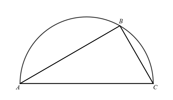
A triangle in a semicircle 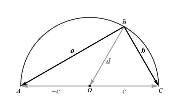
A triangle in a semicircle with vectors Proof (using vectors). Assume that \(A\), \(B\), and \(C\) are points on a circle with diameter \(\overline{AC}.\) Our goal is to prove that the line segments \(\overline{BA}\) and \(\overline{BC}\) are orthogonal. The dot product of vectors is an efficient tool for proving orthogonality. Therefore we use vectors in this proof.
Since \(\overline{AC}\) is a diameter of a circle, this circle's center is the midpoint of \(\overline{AC}.\) Denote this midpoint by \(O.\) Introduce the following vectors by their representative oriented line segments: \[ \mathbf{a}=\overrightarrow{BA}, \quad \mathbf{b}=\overrightarrow{BC}, \quad \mathbf{c}=\overrightarrow{OC}, \quad \text{and} \quad \mathbf{d}=\overrightarrow{BO}. \] Since \(O\) is the midpoint of \(\overline{AC},\) we have that the vector \(-\mathbf{c}\) is represented by \(\overrightarrow{OA}.\) The following algebraic relationships hold among the vectors that we introduced: \begin{align*} \mathbf{a} & = \mathbf{d} - \mathbf{c} \\ \mathbf{b} & = \mathbf{d} + \mathbf{c}. \end{align*} Since \(O\) is the center of a circle and the points (A\), \(B\), and \(C\) are on that circle, we have \[ \| \mathbf{c} \| = \| \mathbf{d} \|. \] Our goal is to prove that the line segments \(\overline{BA}\) and \(\overline{BC}\) are orthogonal. To prove this, we calculate \begin{align*} \mathbf{a} \cdot \mathbf{b} & = (\mathbf{d} - \mathbf{c})\cdot (\mathbf{d} + \mathbf{c}) \\ & = \mathbf{d} \cdot \mathbf{d} - \mathbf{c} \cdot \mathbf{d} + \mathbf{d} \cdot \mathbf{c} - \mathbf{c} \cdot \mathbf{c} \\ & = \mathbf{d} \cdot \mathbf{d} - \mathbf{d} \cdot \mathbf{c} + \mathbf{d} \cdot \mathbf{c} - \mathbf{c} \cdot \mathbf{c} \\ & = \mathbf{d} \cdot \mathbf{d} - \mathbf{c} \cdot \mathbf{c} \\ & = \| \mathbf{d} \|^2 - \| \mathbf{c} \|^2 \\ & = 0. \end{align*} Consequently, the vectors \(\mathbf{a}\) and \(\mathbf{b}\) are orthogonal. Therefore, the line segments \(\overline{BA}\) and \(\overline{BC}\) are orthogonal. QED
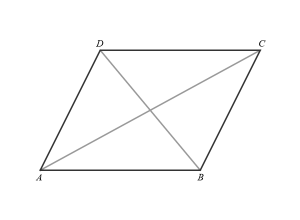
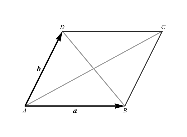
- Today we finished Section 2.3 Dot Product in OpenStax Calculus Volume 3. Do as many problems as you can from 123 to 172. In particular: 124, 125, 127, 130, 131, 135, 137, 138, 141, 142, 143, 145, 147, 148, 150, 151, 153, 154, 155, 157, 158, 159, 161, 165, 168, 170, 172.
- Again, I emphasize that to understand the dot product it is essential to review the Law of Cosine that is taught in trigonometry classes. Here is my webpage with a proof of the Law of Cosines and its connection to dot product.
-
An important application of dot product is the calculation of the orthogonal projection.
Here is my presentation of the orthogonal projection of \(\mathbf{v}\) onto \(\mathbf{u}.\) Given two nonzero vectors \(\mathbf{u}\) and \(\mathbf{v}\), the orthogonal projection of \(\mathbf{v}\) onto \(\mathbf{u}\) is a special scaling of \(\mathbf{u}\), call it \[ \alpha \mkern1mu \mathbf{u}, \qquad \alpha \in \mathbb{R}, \] which has a very special property that the difference \[ \mathbf{v} - \alpha \mkern1mu \mathbf{u} \qquad \text{is orthogonal to} \qquad \mathbf{u}. \] Using the orthogonality stated on the line above, we can calculate \(\alpha\) in terms of \(\mathbf{u}\) and \(\mathbf{v}\): \[ \bigl( \mathbf{v} - \alpha \mkern1mu\mathbf{u}\bigr) \cdot \mathbf{u} = 0. \] Now we use the distributivity property of the dot product to get \[ \mathbf{v} \cdot \mathbf{u} - \alpha \mkern1mu (\mathbf{u} \cdot \mathbf{u}) = 0. \] The last equality we can solve for \(\alpha\): \[ \alpha = \frac{\mathbf{v} \cdot \mathbf{u}}{\mathbf{u} \cdot \mathbf{u}}. \] Now we have the formula for the projection vector of \(\mathbf{v}\) onto \(\mathbf{u}\): \[ \operatorname{proj}_{\mathbf{u}} (\mathbf{v}) = \frac{\mathbf{v} \cdot \mathbf{u}}{\mathbf{u} \cdot \mathbf{u}}\ \mathbf{u} = \frac{\mathbf{v} \cdot \mathbf{u}}{\|\mathbf{u}\|^2} \ \mathbf{u} \]
Now I can write a formula in which we see what is so special about the projection vector of \(\mathbf{v}\) onto \(\mathbf{u}\): \[ \mathbf{v} = \underbrace{\frac{\mathbf{v} \cdot \mathbf{u}}{\|\mathbf{u}\|^2}\,\mathbf{u}}_{\text{a multiple of } \mathbf{u}} + \underbrace{ \left(\mathbf{v} - \frac{\mathbf{v} \cdot \mathbf{u}}{\|\mathbf{u}\|^2}\,\mathbf{u} \right)}_{\text{orthogonal to } \mathbf{u}} \]
-
Orthogonal projections \(\operatorname{proj}_{\mathbf{u}}(\mathbf{v})\) and related vectors in color
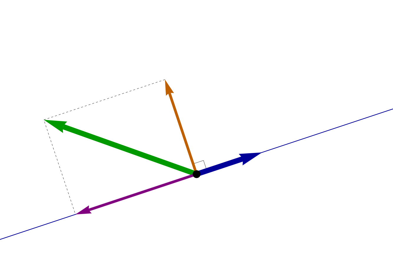
The vector \(\mathbf{u}\) is blue, \(\mathbf{v}\) is green, \(\operatorname{proj}_{\mathbf{u}}(\mathbf{v})\) is dark magenta, \(\mathbf{v}- \operatorname{proj}_{\mathbf{u}}(\mathbf{v})\) is orange, 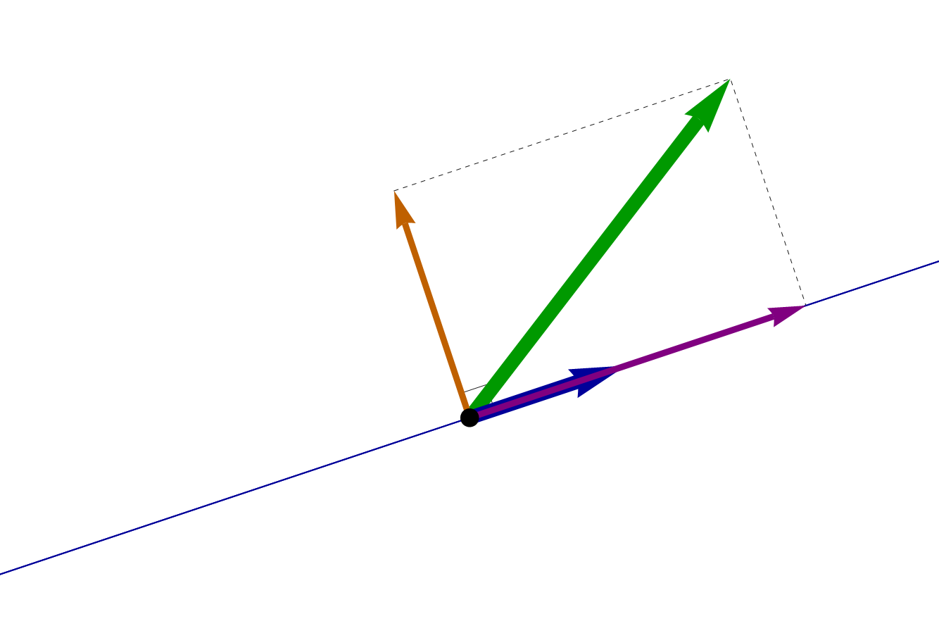
The vector \(\mathbf{u}\) is blue, \(\mathbf{v}\) is green, \(\operatorname{proj}_{\mathbf{u}}(\mathbf{v})\) is dark magenta, \(\mathbf{v}- \operatorname{proj}_{\mathbf{u}}(\mathbf{v})\) is orange,
The animation below illustrates the fact that the projection \(\operatorname{proj}_{\mathbf{u}}(\mathbf{v})\) does not change when \(\mathbf{u}\) is replaced by its nonzero scalar multiple.
-
The Definition of the projection vector on page 140 is confused and formula (2.7) is wrong. Below is a snippet from the definition.
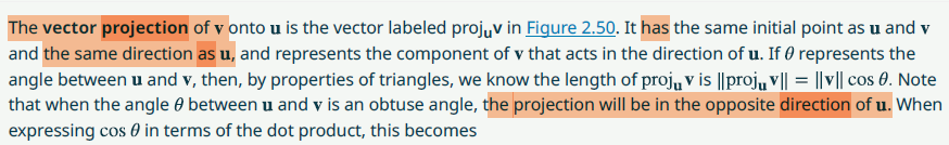 Reading just the orange words, one does not know whether the projection is in the same direction as \(\mathbf{u}\), or it can also be in the opposite direction of \(\mathbf{u}.\) In fact, if the angle between \(\mathbf{v}\) and \(\mathbf{u}\) is acute, then the projection of \(\mathbf{v}\) onto \(\mathbf{u}\) points in the same direction as \(\mathbf{u}\), and if the angle between \(\mathbf{v}\) and \(\mathbf{u}\) is obtuse, then the projection of \(\mathbf{v}\) onto \(\mathbf{u}\) points in the opposite direction of \(\mathbf{u}.\) The projection of \(\mathbf{v}\) onto \(\mathbf{u}\) is always colinear with \(\mathbf{u}.\) That is, it is a scalar multiple of \(\mathbf{u}.\)
Below is the snippet of (2.7) on page 140:
 This is quite confusing. When you look at (2.7), on the left-hand side is a vector, while on the right-hand side is a scalar. They cannot be equal. Vector can never equal a scalar. I was not familiar with the concept scalar projection of \(\mathbf{v}\) onto \(\mathbf{u}.\) Based on my research, the common meaning of the scalar projection of \(\mathbf{v}\) onto \(\mathbf{u}\) is not the length of the projection, but something a little more complicated. One could say that it is the signed length; it is the length when the projection and \(\mathbf{u}\) point in the same direction and it is the opposite of the length when the projection and \(\mathbf{u}\) point in different directions. Or it is the scalar that we use to scale the unit vector of \(\mathbf{u}\) to get the projection.
So, the book is wrong for using the word "length," in the sentence with (2.7), but the formula for \(\operatorname{comp}_{\mathbf{u}} \mathbf{v}\) is correct when one removes \(\operatorname{proj}_{\mathbf{u}} \mathbf{v}.\)
Here is an explanation of \(\operatorname{comp}_{\mathbf{u}} \mathbf{v}\), starting from the formula for \(\operatorname{proj}_{\mathbf{u}} \mathbf{v}\): \[ \operatorname{proj}_{\mathbf{u}}\mkern-5mu \mathbf{v} = \frac{\mathbf{v}\cdot\mathbf{u}}{\|\mathbf{u}\|^2}\,\mathbf{u} = \frac{\mathbf{v}\cdot\mathbf{u}}{\|\mathbf{u}\|}\,\left(\frac{1}{\|\mathbf{u}\|} \mathbf{u}\right) = \underbrace{ \frac{\mathbf{v}\cdot\mathbf{u}}{\|\mathbf{u}\|}}_{ \operatorname{comp}_{\mathbf{u}}\mkern-5mu\mathbf{v}} \mkern 7mu \underbrace{\left(\frac{1}{\|\mathbf{u}\|} \mathbf{u}\right)}_{\begin{array}{c} \text{the unit } \\ \text{vector of} \ \mathbf{u} \end{array}}. \]
-
Theorem about the diagonals in a deltoid. (A common name for a deltoid is a kite.)
If \(ABCD\) is a deltoid with vertices \(A, B, C, D\), as shown below, then its diagonals \(\overline{AC}\) and \(\overline{BD}\) are perpendicular.
Definition of a deltoid. A quadrilateral \(ABCD\) is called a deltoid if and only if it has two pairs of adjacent sides of equal length: \(|\overline{AB}| = |\overline{AD}|\) and \(|\overline{CB}| = |\overline{CD}|\).
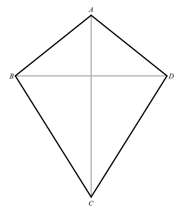
Deltoid \(ABCD\) 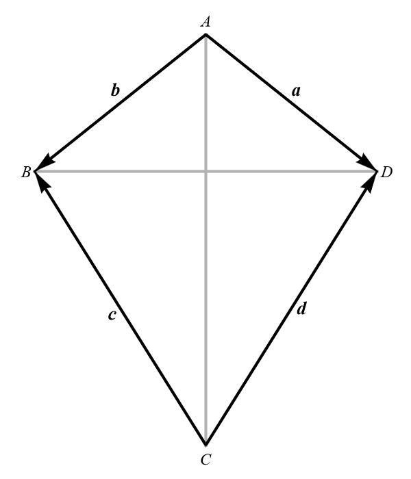
Deltoid \(ABCD\) with vectors Proof (using vectors). Step 1. Introduce the following vectors by their representative line segments: \(\mathbf{a} = \overrightarrow{AD}\), \(\mathbf{b} = \overrightarrow{AB}\), \(\mathbf{c} = \overrightarrow{CB}\), and \(\mathbf{d} = \overrightarrow{CD}.\) Assume that \(|\overline{AB}| = |\overline{AD}|\) and \(|\overline{CB}| = |\overline{CD}|.\) With the vectors introduced, we assume that \[ \|\mathbf{a}\| = \|\mathbf{b}\| \quad \text{and} \quad \|\mathbf{c}\| = \|\mathbf{d}\|. \] Since \[ \mathbf{a} - \mathbf{d} + \mathbf{c} - \mathbf{b} = \mathbf{0}, \] we have that \[ \mathbf{a} - \mathbf{b} = \mathbf{d} - \mathbf{c}, \] and \[ \mathbf{a} - \mathbf{d} = \mathbf{b} - \mathbf{c}. \] The oriented line segment \(\overrightarrow{AC}\) is on one diagonal and it represents the vector \(\mathbf{a} - \mathbf{d} = \mathbf{b} - \mathbf{c}.\) The oriented line segment \(\overrightarrow{BD}\) is on the other diagonal and it represents the vector \(\mathbf{a} - \mathbf{b} = \mathbf{d} - \mathbf{c}.\) Next we will calculate the dot product \[ (\mathbf{a} - \mathbf{b}) \cdot (\mathbf{a} - \mathbf{d}). \]
Step 2. Before calculating this dot product, we establish the following useful equality: \begin{align*} \mathbf{a} - \mathbf{b} & = \frac{1}{2} (\mathbf{a} - \mathbf{b}) + \frac{1}{2} (\mathbf{a} - \mathbf{b}) \\ & = \frac{1}{2} (\mathbf{a} - \mathbf{b}) + \frac{1}{2} (\mathbf{d} - \mathbf{c}) \\ & = \frac{1}{2} (\mathbf{a} + \mathbf{d}) - \frac{1}{2} (\mathbf{b} + \mathbf{c}). \end{align*} Hence we have \[ \mathbf{a} - \mathbf{b} = \frac{1}{2} (\mathbf{a} + \mathbf{d}) - \frac{1}{2} (\mathbf{b} + \mathbf{c}). \]
Step 3. We use this equality to calculate \begin{align*} (\mathbf{a} - \mathbf{b}) \cdot (\mathbf{a} - \mathbf{d}) & = \left(\frac{1}{2} (\mathbf{a} + \mathbf{d}) - \frac{1}{2} (\mathbf{b} + \mathbf{c}) \right) \cdot (\mathbf{a} - \mathbf{d}) \\ & = \frac{1}{2} (\mathbf{a} + \mathbf{d}) \cdot (\mathbf{a} - \mathbf{d}) - \frac{1}{2} (\mathbf{b} + \mathbf{c}) \cdot (\mathbf{a} - \mathbf{d}) \\ & = \frac{1}{2} \bigl( \|\mathbf{a}\|^2 - \|\mathbf{d}\|^2 \bigr) - \frac{1}{2} (\mathbf{b} + \mathbf{c}) \cdot (\mathbf{b} - \mathbf{c}) \\ & = \frac{1}{2} \bigl( \|\mathbf{a}\|^2 - \|\mathbf{d}\|^2 \bigr) - \bigl( \|\mathbf{b}\|^2 - \|\mathbf{c}\|^2 \bigr) \\ & = \frac{1}{2} \bigl( \|\mathbf{a}\|^2 - \|\mathbf{b}\|^2 \bigr) + \frac{1}{2} \bigl( \|\mathbf{c}\|^2 - \|\mathbf{d}\|^2 \bigr) \\ \end{align*} Since we assume \[ \|\mathbf{a}\| = \|\mathbf{b}\| \quad \text{and} \quad \|\mathbf{c}\| = \|\mathbf{d}\|, \] we have \[ (\mathbf{a} - \mathbf{b}) \cdot (\mathbf{a} - \mathbf{d}) = \frac{1}{2} \bigl( \|\mathbf{a}\|^2 - \|\mathbf{b}\|^2 \bigr) + \frac{1}{2} \bigl( \|\mathbf{c}\|^2 - \|\mathbf{d}\|^2 \bigr) = 0. \] Thus, the vectors \(\mathbf{a} - \mathbf{b}\) and \(\mathbf{a} - \mathbf{d}\) are orthogonal. Therefore, the diagonals are orthogonal. QED.
-
Varignon's Theorem
Let \(ABCD\) be a quadrilateral with vertices \(A, B, C, D\) and denote by \(A'\) the midpoint of \(\overline{AB}\), by \(B'\) the midpoint of \(\overline{BC}\), by \(C'\) the midpoint of \(\overline{CD}\), and by \(D'\) the midpoint of \(\overline{DA}\), as pictured below. Then \(A'B'C'D'\) is a parallelogram.
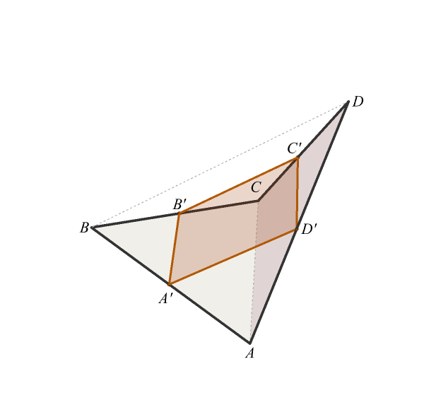
Varignon's Theorem 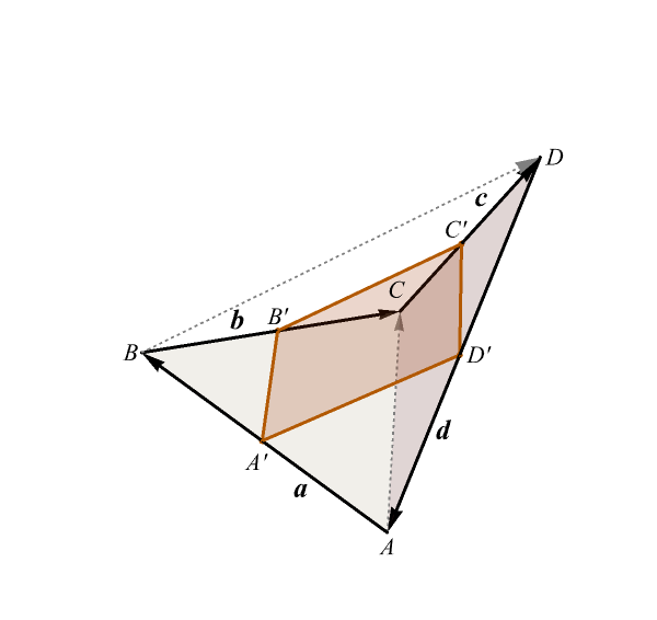
Varignon's Theorem with vectors Proof (using vectors). Step 1. Introduce the following vectors by their representative line segments: \(\mathbf{a} = \overrightarrow{AB}\), \(\mathbf{b} = \overrightarrow{BC}\), \(\mathbf{c} = \overrightarrow{CD}\), and \(\mathbf{d} = \overrightarrow{DA}.\) Since \[ \mathbf{a} + \mathbf{b} + \mathbf{c} + \mathbf{d} = \mathbf{0}, \] we have that \[ \mathbf{b} + \mathbf{c} = - (\mathbf{a} + \mathbf{d}), \] (this vector is represented by the oriented line segment \(\overrightarrow{BD}\)) and \[ \mathbf{a} + \mathbf{b} = -(\mathbf{c} + \mathbf{d}). \] (this vector is represented by the oriented line segment \(\overrightarrow{AC}\)).
Step 2. In triangle \(AA'D'\) we have that the oriented line segment \(\overrightarrow{A'D'}\) represents the vector \(-\frac{1}{2}(\mathbf{a} + \mathbf{d}).\) In triangle \(CB'C'\) we have that the oriented line segment \(\overrightarrow{B'C'}\) represents the vector \(\frac{1}{2}(\mathbf{b} + \mathbf{c}).\) Since we have \[ -\frac{1}{2}(\mathbf{a} + \mathbf{d}) = \frac{1}{2}(\mathbf{b} + \mathbf{c}), \] the oriented line segments \(\overrightarrow{A'D'}\) and \(\overrightarrow{B'C'}\) are equivalent. That is they are parallel and have equal length.
Step 3. In triangle \(BA'B'\) we have that the oriented line segment \(\overrightarrow{A'B'}\) represents the vector \(\frac{1}{2}(\mathbf{a} + \mathbf{b}).\) In triangle \(DD'C'\) we have that the oriented line segment \(\overrightarrow{D'C'}\) represents the vector \(-\frac{1}{2}(\mathbf{d} + \mathbf{c}).\) Since we have \[ -\frac{1}{2}(\mathbf{c} + \mathbf{d}) = \frac{1}{2}(\mathbf{a} + \mathbf{b}), \] the oriented line segments \(\overrightarrow{A'B'}\) and \(\overrightarrow{D'C'}\) are equivalent. That is they are parallel and have equal length.
Conclusion. We proved that the line segments \(\overline{A'D'}\) and \(\overline{B'C'}\) are parallel and have equal length and that the line segments \(\overline{A'B'}\) and \(\overline{D'C'}\) are parallel and have equal length. Therefore, \(A'B'C'D'\) is a parallelogram. QED.
- We finished Section 2.2 Vectors in Three Dimensions today.
- Tomorrow we will do Section 2.3 Dot Product in OpenStax Calculus Volume 3. Do as many problems as you can from 123 to 172. In particular: 124, 125, 127, 130, 131, 135, 137, 138, 141, 142, 143, 145, 147, 148, 150, 151, 153, 154, 155, 157, 158, 159, 161, 165, 168, 170, 172.
- To understand the dot product it is very useful to review the Law of Cosine that is taught in trigonometry classes. Since it is very important, I wrote a webpage for your convenience. Here is a proof of the Law of Cosines and its connection to dot product.
- On Friday we started Section 2.2 Vectors in Three Dimensions in OpenStax Calculus Volume 3. Do as many problems as you can from 61 to 109. In particular: 61-68, 70, 73, 76, 79, 81, 86, 88, 91, 93, 94, 100, 104, 107-109.
-
A compass rose is a common tool for communicating direction in navigation. The compass rose below shows 32 distinct directions. Here are the names of all 32 directions:
E - East EbN - East-by-North ENE - East-Northeast NEbE - Northeast-by-East NE - Northeast NEbN - Northeast-by-North NNE - North-Northeast NbE - North-by-East N - North NbW - North-by-West NNW - North-Northwest NWbN - Northwest-by-North NW - Northwest NWbW - Northwest-by-West WNW - West-Northwest WbN - West-by-North W - West WbS - West-by-South WSW - West-Southwest SWbW - Southwest-by-West SW - Southwest SWbS - Southwest-by-South SSW - South-Southwest SbW - South-by-West S - South SbE - South-by-East SSE - South-Southeast SEbS - Southeast-by-South SE - Southeast SEbE - Southeast-by-East ESE - East-Southeast EbS - East-by-South 
-
The role played by the compass rose in navigation, when we deal with vectors, is played by the unit circle in a coordinate plane.
Below, I show the unit circle with 32 marked angles and their corresponding cosine and sine values. Note, however, that the angles on the compass rose are not the same as those on the unit circle: the compass rose uses angles that are multiples of \(\pi/16\) (11.25 degrees).
For example, if we are given a vector \(\bigl\langle -1, \sqrt{3} \bigr\rangle\), we calculate the corresponding unit vector in the same direction: \(\bigl\langle -1/2, \sqrt{3}/2 \bigr\rangle\); then calculate the angle \(\theta\) such that \(\cos\theta = -1/2, \sin\theta = \sqrt{3}/2\); that is the angle \(\theta = 2 \pi /3\) and we state that the direction of the vector \(\bigl\langle -1, \sqrt{3} \bigr\rangle\) makes the angle of \(2 \pi /3\) with the positive direction of the horizontal axes.
Although it is not done in mathematics classes, having calculated this angle \(2 \pi /3\) or 120 degrees, we can calculate: \(120/11.25 \approx 10.6667.\) This tells us that the vector \(\bigl\langle -1, \sqrt{3} \bigr\rangle\) points in the direction between NNW - North-Northwest and NWbN - Northwest-by-North, a little closer to Northwest-by-North.
Click here to get a pdf file.
Mouse-over the image for a simplified version.
-
Here are a compass rose and the unit circle next to each other:

-
I made some progress on calculating volume of an antiprism whose base is a regular \(n\)-gon and with a given height. For that I use the fact that such an antiprism can be split in \(2n\) congruent pieces. Then I just calculate the volume of one piece. It is like advising a birthday party how to cut a cake in the shape of an antiprism.
Hover your mouse over an image to see the animation.
Cutting an antiprism shaped cake with a pentagonal base. 
Cutting an antiprism shaped cake with a hexagonal base. 
One of 10 pieces of a pentagonal antiprism. 
One of 12 pieces of a hexagonal antiprism.
Cutting an antiprism shaped cake with a square base. 
Cutting an antiprism shaped cake with an equilateral triangle as a base. 
One of 8 pieces of a square antiprism. 
One of 6 pieces of a triangular antiprism.
- The information sheet (updated)
-
The main sources for today class are:
- We first study Vectors. I started writing a webpage to present my vision of the topic Vectors in Two and Three Dimensions.
- In OpenStax Calculus Volume 3 read Section 2.1 Vectors in the Plane and do as many problems as you can from 1 to 44. (This is the primary source for this topic.)
- In Calculus Textbook read Vectors and Dot Product. You can skip Example 3 from medicine.
-
Since we will be working in three-dimensional space, let's begin by reviewing some foundational geometric terminology. The table below pairs common 2D shapes with their 3D counterparts.
2-dimensional object: square rectangle parallelogram circle disk ellipse 3-dimensional object: cube cuboid parallelepiped sphere ball ellipsoid Most of these terms should be familiar. I would like to point out the less frequently used term the cuboid, which is the 3D version of a rectangle. You may know it as a "rectangular prism" or a box 📦. I like the term cuboid; the reason: so prominent object should have its own name, not share it with the family of prisms or a packaging item. The cuboid is a convenient, concise and precise name for a very common shape. As the picture below shows, the term cuboid is used in geometry instruction, even at the primary school level.
- I recommend that you always check Wikipedia and other web pages related to the topics that we study. Usually Wikipedia pages are very informative. However, the Wikipedia page for cuboid is strange. The definition given for cuboid on this page is far too technical and difficult to understand. This Wikipedia entry lists the following alternative names for this concept: rectangular box, rectangular hexahedron, right rectangular prism, and rectangular parallelepiped.