 My talk
was a celebration of this discovery.
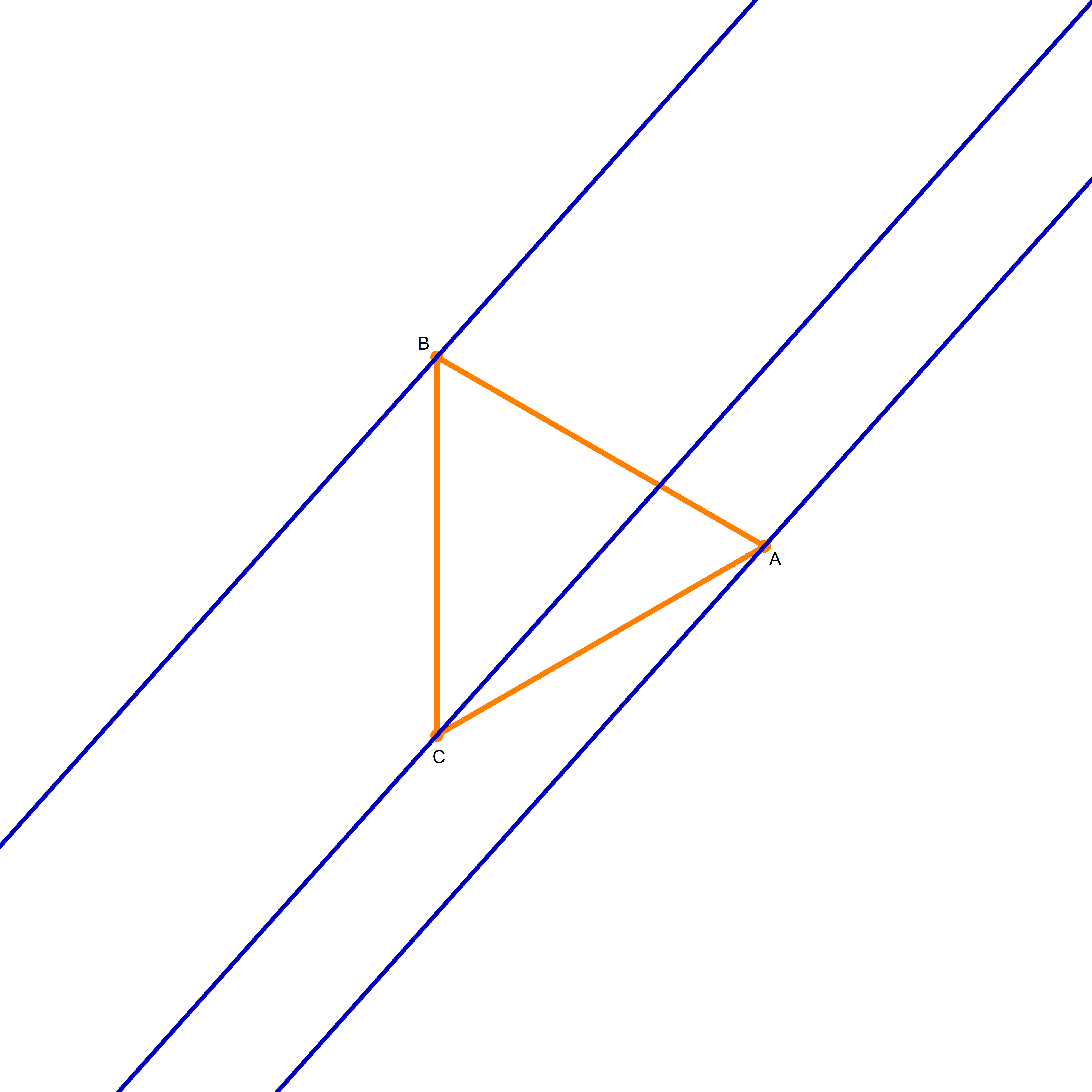
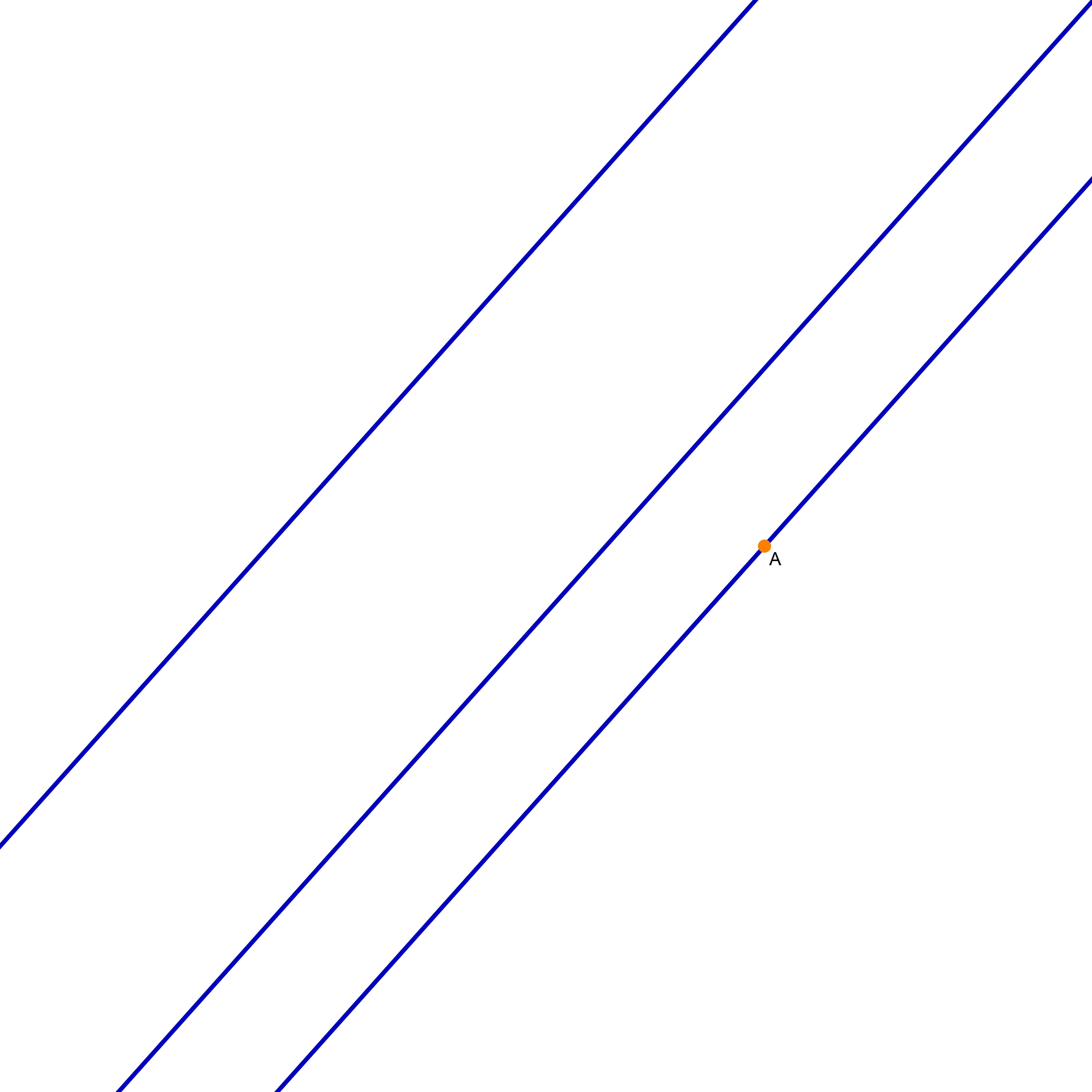
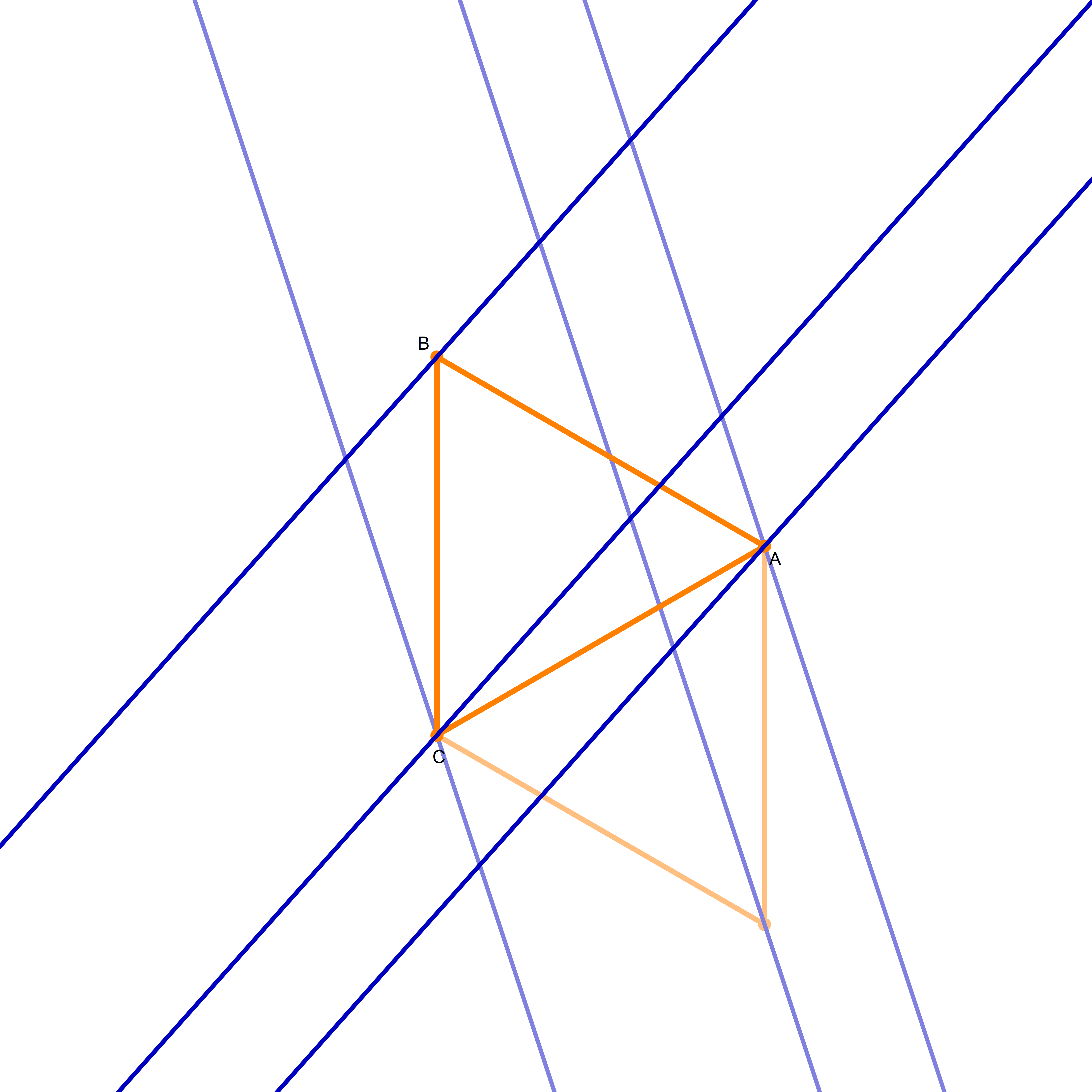
 I am not sure if that is explained on the Wikipedia site straightedge and compass construction but to solve the given problem one needs to know that there exists a straightedge and compass construction which will produce a rotation of a given line by the angle of $\pi/3$ about a given point. Below is the final scene of the rotation in the preceding animation. This final scene contains the solution.
 My talk
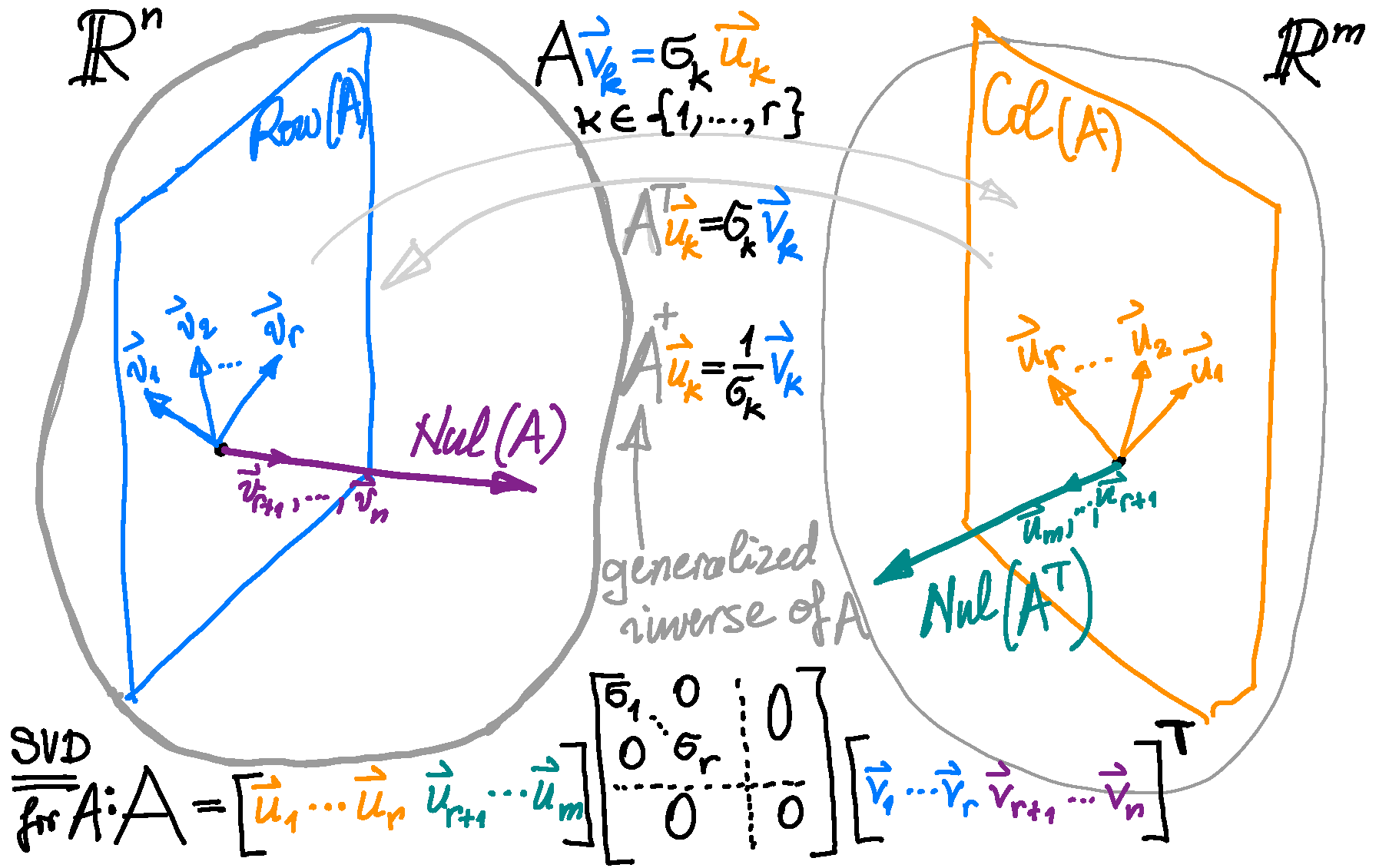
Place the cursor over the image to start the animation.
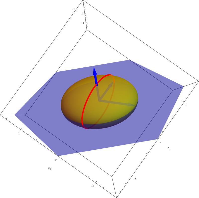
Five of the above level surfaces at different level of opacity.

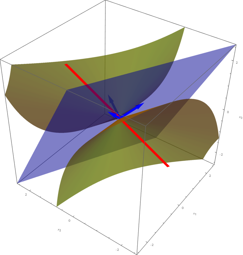 The set
\[
\bigl\{ \mathbf{y} \in \mathbb{R}^3 \, : \, - y_1^2 - y_2^2 + 5 y_3^2 = 1 \bigr\}
\]
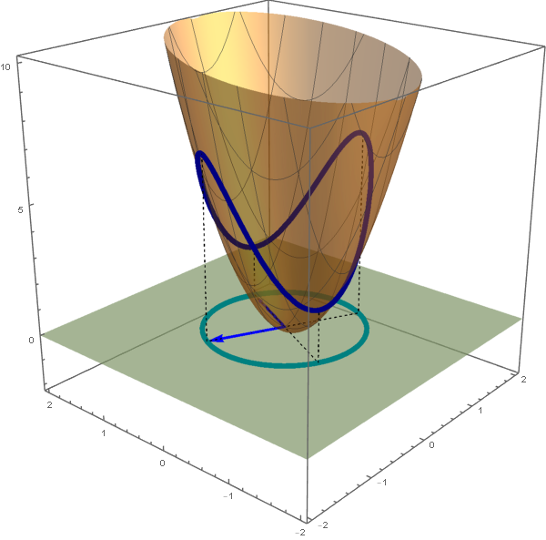
is a rotated two sheet hyperboloid. This two sheet hyperboloid is obtained as the hyperbola $-y_1^2 + 5 y_3^2 = 1, y_2 = 0$ rotates about the $y_3$-axis. Consequently, the set equality stated at the beginning of this item with $c=1$ implies that the set
\[
\bigl\{ \mathbf{x} \in \mathbb{R}^3 \, : \, Q(\mathbf{x}) = 1 \bigr\}
\]
is also a rotated two sheet hyperboloid. This hyperboloid is obtained as a hyperbola in the plane spanned by the vectors
\[
\left[\!
\begin{array}{c}
-\frac{1}{\sqrt{2}} \\ 0 \\ \frac{1}{\sqrt{2}}
\end{array}
\!\right], \quad
\left[\!
\begin{array}{c}
\frac{1}{\sqrt{6}} \\ \frac{2}{\sqrt{6}} \\ \frac{1}{\sqrt{6}}
\end{array}
\!\right]
\]
rotates about the vector
\[
\left[\!
\begin{array}{c}
\frac{1}{\sqrt{6}} \\ \frac{2}{\sqrt{6}} \\ \frac{1}{\sqrt{6}}
\end{array}
\!\right].
\]
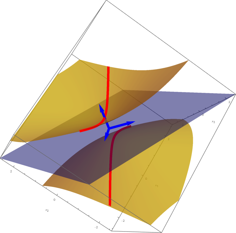 The set
\[
\bigl\{ \mathbf{y} \in \mathbb{R}^3 \, : \, - y_1^2 - y_2^2 + 5 y_3^2 = -1 \bigr\}
\]
is a rotated one sheet hyperboloid. This hyperboloid is obtained as the hyperbola $-y_2^2 + 5 y_3^2 = -1, y_1 = 0$ rotates about $y_3$-axis. The set equality stated at the beginning of this item with $c=-1$ implies that the set
\[
\bigl\{ \mathbf{x} \in \mathbb{R}^3 \, : \, Q(\mathbf{x}) = -1 \bigr\}
\]
is also a rotated one sheet hyperboloid. This hyperboloid is obtained as a hyperbola in the plane spanned by the vectors
\[
\left[\!
\begin{array}{c}
\frac{1}{\sqrt{3}} \\ -\frac{1}{\sqrt{3}} \\ \frac{1}{\sqrt{3}}
\end{array}
\!\right], \quad
\left[\!
\begin{array}{c}
\frac{1}{\sqrt{6}} \\ \frac{2}{\sqrt{6}} \\ \frac{1}{\sqrt{6}}
\end{array}
\!\right]
\]
rotates about the vector
\[
\left[\!
\begin{array}{c}
\frac{1}{\sqrt{6}} \\ \frac{2}{\sqrt{6}} \\ \frac{1}{\sqrt{6}}
\end{array}
\!\right].
\]
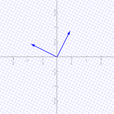 With the change of coordinates
\[
\mathbf{y} = \underset{\mathcal{B}\leftarrow\mathcal{E}}{P} \mathbf{x}, \qquad
\mathbf{x} = \underset{\mathcal{E}\leftarrow\mathcal{B}}{P} \mathbf{y},
\]
the quadratic form $Q$ simplifies as follows
\[
6 x_1^2 - 4 x_2 x_1 + 3 x_2^2 = 2 y_1^2 + 7 y_2^2.
\]
Since clearly $2 y_1^2 + 7 y_2^2 \geq 0$ for all $y_1, y_2 \in \mathbb{R}$ and $2 y_1^2 + 7 y_2^2 = 0$ if and only if $(y_1,y_2) =(0,0).$ In conclusion, the given quadratic form is positive definite.
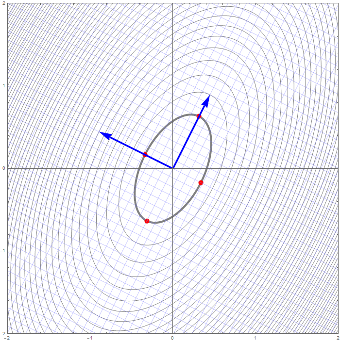
 With the change of coordinates
\[
\mathbf{y} = \underset{\mathcal{B}\leftarrow\mathcal{E}}{P} \mathbf{x}, \qquad
\mathbf{x} = \underset{\mathcal{E}\leftarrow\mathcal{B}}{P} \mathbf{y},
\]
the quadratic form $Q$ simplifies as follows
\[
x_1^2 + 6 x_2 x_1 + x_2^2 = 4 y_1^2 - 2 y_2^2.
\]
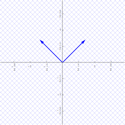
Clearly $4 y_1^2 - 2 y_2^2$ is an indefinite form taking the value $4$ at $(y_1,y_2) = (1,0)$ and the value $-2$ at $(y_1,y_2) = (0,1).$
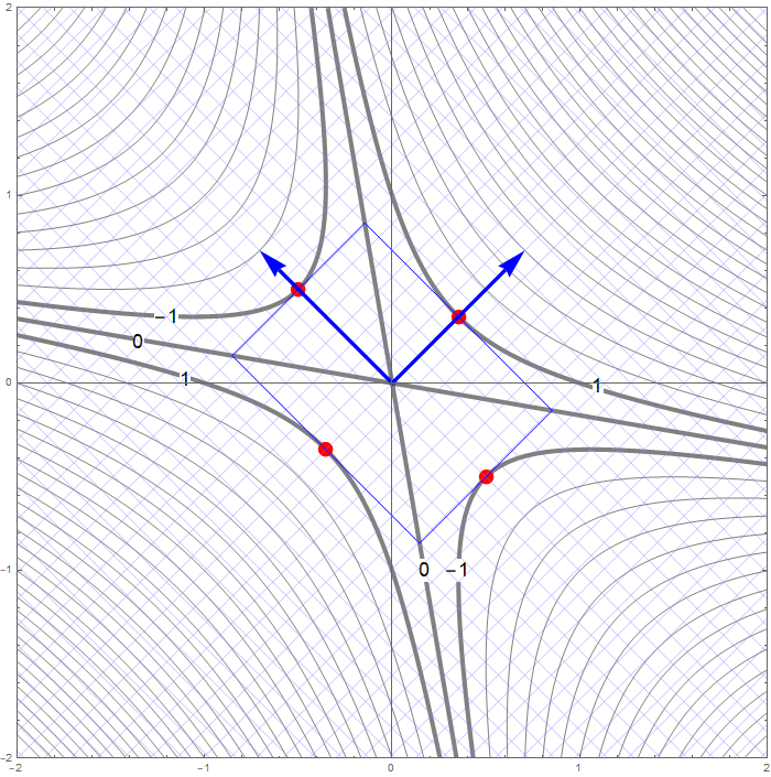
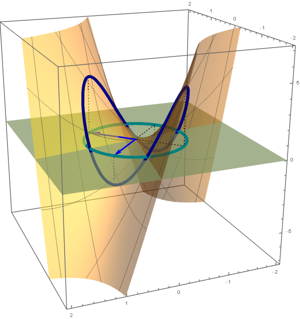
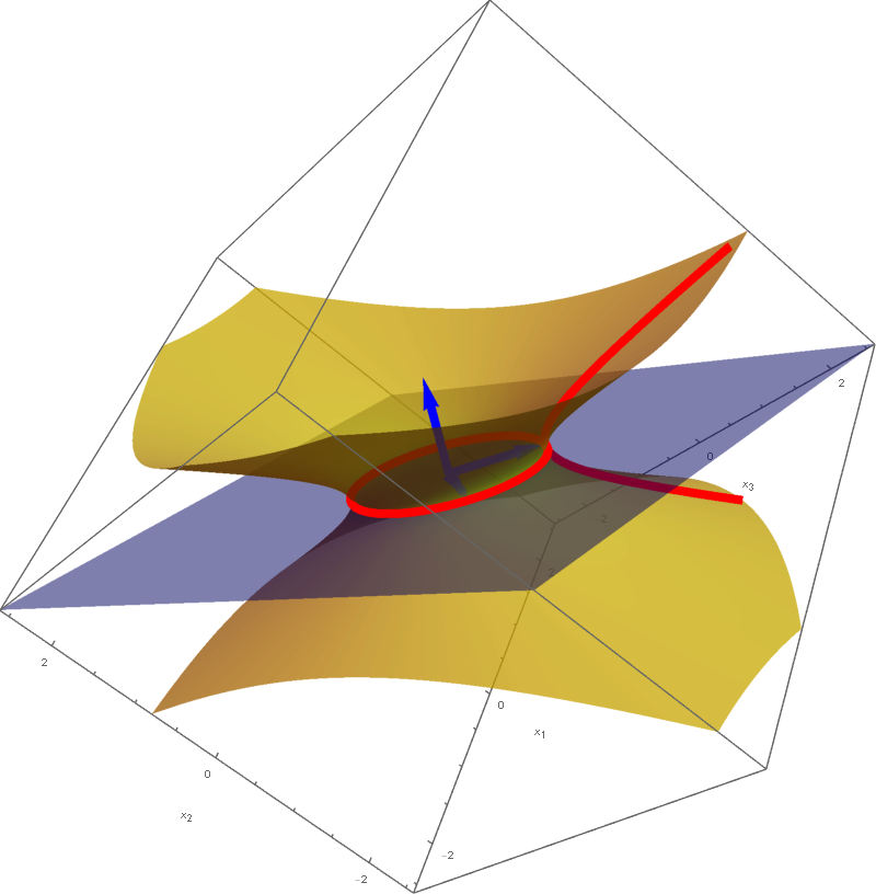
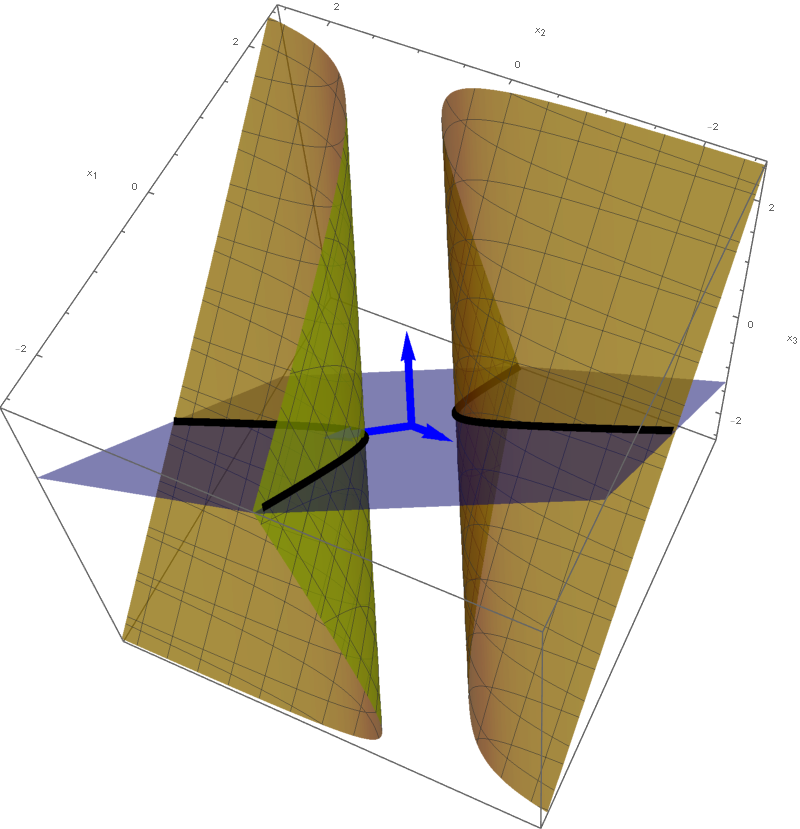 The set
\[
\bigl\{ \mathbf{x} \in \mathbb{R}^3 \, : \, Q(\mathbf{x}) = -1 \bigr\} = \bigl\{ \mathbf{y} \in \mathbb{R}^3 \, : \, - 3 y_1^2 + 3 y_2^2 = -1 \bigr\}
\]
is a hyperbolic cylinder. The equation $- 3 y_1^2 + 3 y_2^2 = -11$ represents a hyperbola in the plane spanned by the vectors
\[
\left[\!
\begin{array}{c}
-\frac{1}{3} \\ -\frac{2}{3} \\ \frac{2}{3}
\end{array}
\!\right] \quad \text{and} \quad \left[\!
\begin{array}{c}
-\frac{2}{3} \\ \frac{2}{3} \\ \frac{1}{3}
\end{array}
\!\right] \quad \text{coordinates relative to} \quad \mathcal{E}.
\]
The cylinder is formed by the parallel lines that go through the points on the hyperbola and are orthogonal to the plane spanned by the above two vectors.
In the image below I give a graphical representation of the above quadruplicity. The red dot represents the zero quadratic form, the green region represents the positive semidefinite quadratic forms, the blue region represents the negative semidefinite quadratic forms and the cyan region represents the indefinite quadratic forms.
In the image above, the dark green region represents the positive definite quadratic forms and the dark blue region represents the negative definite quadratic forms. These two regions are not parts of the above quadruplicity.
The Complex Numbers. A complex number is commonly represented as $z = x + i y$ where $i$ is the imaginary unit with the property $i^2 = -1$ and $x$ and $y$ are real numbers. The real number $x$ is called the real part of $z$ and the real number $y$ is called the imaginary part of $z.$ A real number is a special complex numbers whose imaginary part is $0.$ The set of all complex numbers is denoted by $\mathbb C.$
The Complex Conjugate. By $\overline{z}$ we denote the complex conjugate of $z$. The complex conjugate of $z = x+i y$ is the complex number $\overline{z} = x - i y.$ That is, the complex conjugate $\overline{z}$ is the complex numer which has the same real part as $z$ and the imaginary part of $\overline{z}$ is the opposite of the imaginary part of $z.$ Since $-0 = 0$, a comlex number $z$ is real if and only if $\overline{z} = z.$ The operation of complex conjugation respects the algebraic operations with complex numbers: \[ \overline{z + w} = \overline{z} + \overline{w}, \quad \overline{z - w} = \overline{z} - \overline{w}, \quad \overline{z\, w} = \overline{z}\, \overline{w}. \]
The Modulus. Let $z = x + i y$ be a complex number. Here $x$ is the real part of $z$ and $y$ is the imaginary part of $z.$ The modulus of $z$ is the nonnegative number $\sqrt{x^2+y^2}.$ The modulus of $z$ is denoted by $|z|.$ Clearly, $|z|^2 = z\overline{z}$.
Vectors with Complex Entries. Let $\mathbf v$ be a vector with complex entries. By $\overline{\mathbf{v}}$ we denote the vector whose entries are complex conugates of the corresponding entries of $\mathbf v.$ That is, \[ \mathbf v = \left[\begin{array}{c} v_1 \\ \vdots \\ v_n \end{array} \right], \qquad \overline{\mathbf v} = \left[\begin{array}{c} \overline{v}_1 \\ \vdots \\ \overline{v}_n \end{array} \right]. \] The following calculation for a vector with complex entries is often useful \[ \mathbf{v}^\top \overline{\mathbf{v}} = \bigl[v_1 \ \ v_2 \ \ \cdots \ \ v_n \bigr] \left[\begin{array}{c} \overline{v}_1 \\ \overline{v}_2 \\ \vdots \\ \overline{v}_n \end{array} \right] = \sum_{k=1}^n v_k\, \overline{v}_k = \sum_{k=1}^n |v_k|^2 \geq 0. \] Moreover, \[ \mathbf{v}^\top \overline{\mathbf{v}} = 0 \quad \text{if and only if} \quad \mathbf{v} = \mathbf{0}. \] Equivalently, \[ \mathbf{v}^\top \overline{\mathbf{v}} \gt 0 \quad \text{if and only if} \quad \mathbf{v} \neq \mathbf{0}. \]
Theorem. All eigenvalues of a symmetric matrix are real.
Proof. Let $A$ be a symmetric $n\!\times\!n$ matrix and let $\lambda$ be an eigenvalue of $A$. Let $\mathbf{v} = \bigl[v_1 \ \ v_2 \ \ \cdots \ \ v_n \bigr]^\top$ be a corresponding eigenvector. Then $\mathbf{v} \neq \mathbf{0}.$ We allow the possibility that $\lambda$ and the entries $v_1,$ $v_2,\ldots,$ $v_n$ of $\mathbf{v}$ are complex numbers. Since $\mathbf{v}$ is an eigenvector of $A$ corresponding to $\lambda$ we have \[ A \mathbf{v} = \lambda \mathbf{v}. \] Since $A$ is a symmetric matrix, all the entries of $A$ are real numbers. It follows from the properties of the complex conjugation that taking the complex conjugate of each side of the equality $A \mathbf{v} = \lambda \mathbf{v}$ yields \[ A \overline{\mathbf{v}} = \overline{\lambda} \overline{\mathbf{v}}. \] Since $A$ is symmetric, that is $A=A^\top$, we also have \[ A^\top \overline{\mathbf{v}} = \overline{\lambda} \overline{\mathbf{v}}. \] Multiplying both sides of the last equation by $\mathbf{v}^\top$ we get \[ \mathbf{v}^\top \bigl( A^\top \overline{\mathbf{v}} \bigr) = \mathbf{v}^\top ( \overline{\lambda} \overline{\mathbf{v}}). \] Since $\mathbf{v}^\top A^\top = \bigl(A\mathbf{v}\bigr)^\top$ and $\mathbf{v}^\top ( \overline{\lambda} \overline{\mathbf{v}}) = \overline{\lambda} \mathbf{v}^\top \overline{\mathbf{v}}$ the last displayed equality is equivalent to \[ \bigl(A\mathbf{v}\bigr)^\top \overline{\mathbf{v}} = \overline{\lambda} \mathbf{v}^\top \overline{\mathbf{v}}. \] Since $A \mathbf{v} = \lambda \mathbf{v},$ we further have \[ \bigl(\lambda \mathbf{v}\bigr)^\top \overline{\mathbf{v}} = \overline{\lambda} \mathbf{v}^\top \overline{\mathbf{v}}. \] That is, \[ \tag{*} \lambda \mathbf{v}^\top \overline{\mathbf{v}} = \overline{\lambda} \mathbf{v}^\top \overline{\mathbf{v}}. \] As explained in Vectors with Complex Entries item, $\mathbf{v} \neq \mathbf{0},$ implies $\mathbf{v}^\top \overline{\mathbf{v}} \gt 0.$ Now dividing both sides of equality (*) by $\mathbf{v}^\top \overline{\mathbf{v}} \gt 0$ yields \[ \lambda = \overline{\lambda}. \] As explained in The Complex Conjugate item above, this proves that $\lambda$ is a real number.
Theorem. Eigenspaces of a symmetric matrix which correspond to distinct eigenvalues are orthogonal.
Proof. Let $A$ be a symmetric $n\!\times\!n$ matrix. Let $\lambda$ and $\mu$ be an eigenvalues of $A$ and let $\mathbf{u}$ and $\mathbf{v}$ be a corresponding eigenvector. Then $\mathbf{u} \neq \mathbf{0},$ $\mathbf{v} \neq \mathbf{0}$ and \[ A \mathbf{u} = \lambda \mathbf{u} \quad \text{and} \quad A \mathbf{v} = \mu \mathbf{v}. \] Assume that \[ \lambda \neq \mu. \] Next we calculate the same dot product in two different ways; here we use the fact that $A^\top = A$ and algebra of the dot product. The first calculation: \[ (A \mathbf{u})\cdot \mathbf{v} = (\lambda \mathbf{u})\cdot \mathbf{v} = \lambda (\mathbf{u}\cdot\mathbf{v}) \] The second calculation: \begin{align*} (A \mathbf{u})\cdot \mathbf{v} & = (A \mathbf{u})^\top \mathbf{v} = \mathbf{u}^\top A^\top \mathbf{v} = \mathbf{u} \cdot \bigl(A^\top \mathbf{v} \bigr) = \mathbf{u} \cdot \bigl(A \mathbf{v} \bigr) \\ & = \mathbf{u} \cdot (\mu \mathbf{v} ) = \mu ( \mathbf{u} \cdot \mathbf{v}) \end{align*} Since, \[ (A \mathbf{u})\cdot \mathbf{v} = \lambda (\mathbf{u}\cdot\mathbf{v}) \quad \text{and} \quad (A \mathbf{u})\cdot \mathbf{v} = \mu (\mathbf{u}\cdot\mathbf{v}) \] we conclude that \[ \lambda (\mathbf{u}\cdot\mathbf{v}) - \mu (\mathbf{u}\cdot\mathbf{v}) = 0. \] Therefore \[ ( \lambda - \mu ) (\mathbf{u}\cdot\mathbf{v}) = 0. \] Since we assume that $ \lambda - \mu \neq 0,$ the previous displayed equality yields \[ \mathbf{u}\cdot\mathbf{v} = 0. \] This proves that any two eigenvectors corresponding to distinct eigenvalues are orthogonal. Thus, the eigenspaces corresponding to distinct eigenvalues are orthogonal.
Theorem. A symmetric $2\!\times\!2$ matrix is orthogonally diagonalizable.
Proof. Let $A = \begin{bmatrix} a & b \\ b & d \end{bmatrix}$ be an arbitrary $2\!\times\!2$ be a symmetric matrix. We need to prove that there exists an orthogonal $2\!\times\!2$ matrix $U$ and a diagonal $2\!\times\!2$ matrix $D$ such that $A = UDU^\top.$ The eigenvalues of $A$ are \[ \lambda_1 = \frac{1}{2} \Bigl( a+d - \sqrt{(a-d)^2 + 4 b^2} \Bigr), \quad \lambda_2 = \frac{1}{2} \Bigl( a+d + \sqrt{(a-d)^2 + 4 b^2} \Bigr) \] Since clearly \[ (a-d)^2 + 4 b^2 \geq 0, \] the eigenvalues $\lambda_1$ and $\lambda_2$ are real numbers.
If $\lambda_1 = \lambda_2$, then $(a-d)^2 + 4 b^2 = 0$, and consequently $b= 0$ and $a=d$; that is $A = \begin{bmatrix} a & 0 \\ 0 & a \end{bmatrix}$. Hence $A = UDU^\top$ holds with $U=I_2$ and $D = A$.
Now assume that $\lambda_1 \neq \lambda_2$. Let $\mathbf{u}_1$ be a unit eigenvector corresponding to $\lambda_1$ and let $\mathbf{u}_2$ be a unit eigenvector corresponding to $\lambda_2$. We proved that eigenvectors corresponding to distinct eigenvalues of a symmetric matrix are orthogonal. Since $A$ is symmetric, $\mathbf{u}_1$ and $\mathbf{u}_2$ are orthogonal, that is the matrix $U = \begin{bmatrix} \mathbf{u}_1 & \mathbf{u}_2 \end{bmatrix}$ is orthogonal. Since $\mathbf{u}_1$ and $\mathbf{u}_2$ are eigenvectors of $A$ we have \[ AU = U \begin{bmatrix} \lambda_1 & 0 \\ 0 & \lambda_2 \end{bmatrix} = UD. \] Therefore $A=UDU^\top.$ This proves that $A$ is orthogonally diagonalizable.
Second Proof. Let $A = \begin{bmatrix} a & b \\ b & d \end{bmatrix}$ an arbitrary $2\!\times\!2$ be a symmetric matrix. If $b=0$, then an orthogonal diagonalization is \[ \begin{bmatrix} a & 0 \\ 0 & d \end{bmatrix} = \begin{bmatrix} 1 & 0 \\ 0 & 1 \end{bmatrix}\begin{bmatrix} a & 0 \\ 0 & d \end{bmatrix}\begin{bmatrix} 1 & 0 \\ 0 & 1 \end{bmatrix}. \] Assume that $b\neq0.$ For the given $a,b,c \in \mathbb{R},$ introduce three new coordinates $z \in \mathbb{R},$ $r \in (0,+\infty),$ and $\theta \in (0,\pi)$ such that \begin{align*} z & = \frac{a+d}{2}, \\ r & = \sqrt{\left( \frac{a-d}{2} \right)^2 + b^2}, \\ \cos(2\theta) & = \frac{\frac{a-d}{2}}{r}, \quad \sin(2\theta) = \frac{b}{r}. \end{align*} The reader will notice that these coordinates are very similar to the cylindrical coordinates in $\mathbb{R}^3.$ It is now an exercise in matrix multiplication and trigonometry to calculate \begin{align*} & \begin{bmatrix} \cos(\theta) & -\sin(\theta) \\ \sin(\theta) & \cos(\theta) \end{bmatrix} \begin{bmatrix} z+r & 0 \\ 0 & z-r \end{bmatrix}\begin{bmatrix} \cos(\theta) & \sin(\theta) \\ -\sin(\theta) & \cos(\theta) \end{bmatrix} \\[6pt] & \quad = \begin{bmatrix} \cos(\theta) & -\sin(\theta) \\ \sin(\theta) & \cos(\theta) \end{bmatrix} \begin{bmatrix} (z+r) \cos(\theta) & (z+r) \sin(\theta) \\ (r-z)\sin(\theta) & (z-r) \cos(\theta) \end{bmatrix} \\[6pt] & \quad = \begin{bmatrix} (z+r) (\cos(\theta))^2 - (r-z)(\sin(\theta))^2 & (z+r) \cos(\theta) \sin(\theta) -(z-r) \cos(\theta) \sin(\theta) \\ (z+r) \cos(\theta) \sin(\theta) + (r-z) \cos(\theta) \sin(\theta) & (z+r) (\sin(\theta))^2 + (z-r)(\cos(\theta))^2 \end{bmatrix} \\[6pt] & \quad = \begin{bmatrix} z + r \cos(2\theta) & r \sin(2\theta) \\ r \sin(2\theta) & z - r \cos(2\theta) \end{bmatrix} \\[6pt] & \quad = \begin{bmatrix} \frac{a+d}{2} + \frac{a-d}{2} & b \\ b & \frac{a+d}{2} - \frac{a-d}{2} \end{bmatrix} \\[6pt] & \quad = \begin{bmatrix} a & b \\ b & d \end{bmatrix}. \end{align*}
Theorem. For every positive integer $n$, a symmetric $n\!\times\!n$ matrix is orthogonally diagonalizable.
Proof. This statement can be proved by Mathematical Induction. The base case $n = 1$ is trivial. The case $n=2$ is proved above. To get a feel how mathematical induction proceeds we will prove the theorem for $n=3.$
Let $A$ be a $3\!\times\!3$ symmetric matrix. Then $A$ has an eigenvalue, which must be real. Denote this eigenvalue by $\lambda_1$ and let $\mathbf{u}_1$ be a corresponding unit eigenvector. Let $\mathbf{v}_1$ and $\mathbf{v}_2$ be unit vectors such that the vectors $\mathbf{u}_1,$ Let $\mathbf{v}_1$ and $\mathbf{v}_2$ form an orthonormal basis for $\mathbb R^3.$ Then the matrix $V_1 = \bigl[\mathbf{u}_1 \ \ \mathbf{v}_1\ \ \mathbf{v}_2\bigr]$ is an orthogonal matrix and we have \[ V_1^\top A V_1 = \begin{bmatrix} \mathbf{u}_1^\top A \mathbf{u}_1 & \mathbf{u}_1^\top A \mathbf{v}_1 & \mathbf{u}_1^\top A \mathbf{v}_2 \\[5pt] \mathbf{v}_1^\top A \mathbf{u}_1 & \mathbf{v}_1^\top A \mathbf{v}_1 & \mathbf{v}_1^\top A \mathbf{v}_2 \\[5pt] \mathbf{v}_2^\top A \mathbf{u}_1 & \mathbf{v}_2^\top A \mathbf{v}_1 & \mathbf{v}_2^\top A \mathbf{v}_2 \\\end{bmatrix}. \] Since $A = A^\top$, $A\mathbf{u}_1 = \lambda_1 \mathbf{u}_1$ and since $\mathbf{u}_1$ is orthogonal to both $\mathbf{v}_1$ and $\mathbf{v}_2$ we have \[ \mathbf{u}_1^\top A \mathbf{u}_1 = \lambda_1, \quad \mathbf{v}_j^\top A \mathbf{u}_1 = \lambda_1 \mathbf{v}_j^\top \mathbf{u}_1 = 0, \quad \mathbf{u}_1^\top A \mathbf{v}_j = \bigl(A \mathbf{u}_1\bigr)^\top \mathbf{v}_j = 0, \quad \quad j \in \{1,2\}, \] and \[ \mathbf{v}_2^\top A \mathbf{v}_1 = \bigl(\mathbf{v}_2^\top A \mathbf{v}_1\bigr)^\top = \mathbf{v}_1^\top A^\top \mathbf{v}_2 = \mathbf{v}_1^\top A \mathbf{v}_2. \] Hence, \[ \tag{**} V_1^\top A V_1 = \begin{bmatrix} \lambda_1 & 0 & 0 \\[5pt] 0 & \mathbf{v}_1^\top A \mathbf{v}_1 & \mathbf{v}_1^\top A \mathbf{v}_2 \\[5pt] 0 & \mathbf{v}_1^\top A \mathbf{v}_2 & \mathbf{v}_2^\top A \mathbf{v}_2 \\\end{bmatrix}. \] By the already proved theorem for $2\!\times\!2$ symmetric matrix there exists an orthogonal matrix $\begin{bmatrix} u_{11} & u_{12} \\[5pt] u_{21} & u_{22} \end{bmatrix}$ and a diagonal matrix $\begin{bmatrix} \lambda_2 & 0 \\[5pt] 0 & \lambda_3 \end{bmatrix}$ such that \[ \begin{bmatrix} \mathbf{v}_1^\top A \mathbf{v}_1 & \mathbf{v}_1^\top A \mathbf{v}_2 \\[5pt] \mathbf{v}_1^\top A \mathbf{v}_2 & \mathbf{v}_2^\top A \mathbf{v}_2 \end{bmatrix} = \begin{bmatrix} u_{11} & u_{12} \\[5pt] u_{21} & u_{22} \end{bmatrix} \begin{bmatrix} \lambda_2 & 0 \\[5pt] 0 & \lambda_3 \end{bmatrix} \begin{bmatrix} u_{11} & u_{12} \\[5pt] u_{21} & u_{22} \end{bmatrix}^\top. \] Substituting this equality in (**) and using some matrix algebra we get \[ V_1^\top A V_1 = \begin{bmatrix} 1 & 0 & 0 \\[5pt] 0 & u_{11} & u_{12} \\[5pt] 0 & u_{21} & u_{22} \end{bmatrix} % \begin{bmatrix} \lambda_1 & 0 & 0 \\[5pt] 0 & \lambda_2 & 0 \\[5pt] 0 & 0 & \lambda_3 \end{bmatrix} % \begin{bmatrix} 1 & 0 & 0 \\[5pt] 0 & u_{11} & u_{12} \\[5pt] 0 & u_{21} & u_{22} \end{bmatrix}^\top \] Setting \[ U = V_1 \begin{bmatrix} 1 & 0 & 0 \\[5pt] 0 & u_{11} & u_{12} \\[5pt] 0 & u_{21} & u_{22} \end{bmatrix} \quad \text{and} \quad D = \begin{bmatrix} \lambda_1 & 0 & 0 \\[5pt] 0 & \lambda_2 & 0 \\[5pt] 0 & 0 & \lambda_3 \end{bmatrix} \] we have that $U$ is an orthogonal matrix, $D$ is a diagonal matrix and $A = UDU^\top.$ This proves that $A$ is orthogonally diagonalizable.
 Since this is not Linear Algebra content, I will move (b) in Problem 4 on Assignment 3 to the Background Knowledge.
We will talk more about this in class. We will develop an alternative way of writing matrix $A$ as a linear combination of orthogonal projections onto the eigenspaces of $A$.
The columns of \[ \left[ \begin{array}{ccc} -\frac{2}{3} & \frac{1}{3} & \frac{2}{3} \\ \frac{1}{3} & -\frac{2}{3} & \frac{2}{3} \\ \frac{2}{3} & \frac{2}{3} & \frac{1}{3} \end{array} \right] \] form an orthonormal basis for $\mathbb{R}^3$ which consists of unit eigenvectors of $A.$
The first two columns \[ \left[ \begin{array}{cc} -\frac{2}{3} & \frac{1}{3} \\ \frac{1}{3} & -\frac{2}{3} \\ \frac{2}{3} & \frac{2}{3} \end{array} \right] \] form an orthonormal basis for the eigenspace of $A$ corresponding to $-1.$ The last column \[ \left[ \begin{array}{c} \frac{2}{3} \\ \frac{2}{3} \\ \frac{1}{3} \end{array} \right] \] is an orhonormal basis for the eigenspace of $A$ corresponding to $8.$
The orthogonal projection matrix onto the eigenspace of $A$ corresponding to $-1$ is \[ P_{-1} = \left[ \begin{array}{cc} -\frac{2}{3} & \frac{1}{3} \\ \frac{1}{3} & -\frac{2}{3} \\ \frac{2}{3} & \frac{2}{3} \end{array} \right] \left[ \begin{array}{ccc} -\frac{2}{3} & \frac{1}{3} & \frac{2}{3} \\ \frac{1}{3} & -\frac{2}{3} & \frac{2}{3} \end{array} \right] = \frac{1}{9} \left[ \begin{array}{rrr} 5 & -4 & -2 \\ -4 & 5 & -2 \\ -2 & -2 & 8 \end{array} \right] \]
The orthogonal projection matrix onto the eigenspace of $A$ corresponding to $8$ is \[ P_8 = \left[ \begin{array}{c} \frac{2}{3} \\ \frac{2}{3} \\ \frac{1}{3} \end{array} \right] \left[ \begin{array}{ccc} \frac{2}{3} & \frac{2}{3} & \frac{1}{3} \end{array} \right] = \frac{1}{9} \left[ \begin{array}{rrr} 4 & 4 & 2 \\ 4 & 4 & 2 \\ 2 & 2 & 1 \end{array} \right]. \]
Since the eigenvectors that we used above form a basis for $\mathbb{R}^3$ we have \[ P_{-1} + P_8 = \frac{1}{9} \left[ \begin{array}{rrr} 5 & -4 & -2 \\ -4 & 5 & -2 \\ -2 & -2 & 8 \end{array} \right] + \frac{1}{9} \left[ \begin{array}{rrr} 4 & 4 & 2 \\ 4 & 4 & 2 \\ 2 & 2 & 1 \end{array} \right] = \left[ \begin{array}{rrr} 1 & 0 & 0 \\ 0 & 1 & 0 \\ 0 & 0 & 1 \end{array} \right] = I_3. \]
Mathematica respondsIntegrate[Cos[m t]*Cos[n t], {t, -Pi, Pi}]
 We immediately see that the above formula does not hold for $m=n.$ Next, we exercise our knowledge that for $m, n \in \mathbb{N}$ we have $\sin(m \pi) = 0$ and $\sin(n \pi) = 0$ to verify that
\[
\int_{-\pi}^{\pi} \cos(m t) \, \cos(n t) dt = 0 \quad \text{whenever} \quad m\neq n.
\]
Warning: Mathematica has powerful commands Simplify[] and FullSimplify[] in which we can place assumptions and ask Mathematica to algebraically simplify mathematical expressions. For example,
Unfortunately, Mathematica response to this command is 0. This is clearly wrong when m and n are equal; as shown by evaluatingFullSimplify[ Integrate[Cos[m t]*Cos[n t], {t, -Pi, Pi}], And[n \[Element] Integers, m \[Element] Integers] ]
So, Mathematica is powerful, but one has to exercise critical thinking.FullSimplify[ Integrate[Cos[n t]*Cos[n t], {t, -Pi, Pi}], And[n \[Element] Integers] ]
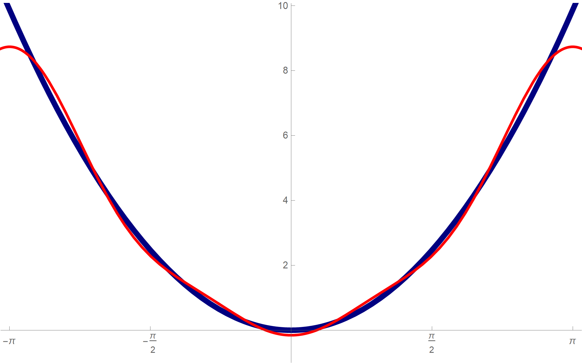
Changing the value of nn in the above Mathematica expression one gets a better approximation.nn = 3; Plot[ {t^2, \[Pi]^2/3*1 + Sum[(4 (-1)^k)/k^2*Cos[k t], {k, 1, nn}]}, {t, -3 Pi, 3 Pi}, PlotPoints -> {100, 200}, PlotStyle -> { {RGBColor[0, 0, 0.5], Thickness[0.01]}, {RGBColor[1, 0, 0], Thickness[0.005]} }, Ticks -> {Range[-2 Pi, 2 Pi, Pi/2], Range[-14, 14, 2]}, PlotRange -> {{-Pi - 0.1, Pi + 0.1}, {-1, Pi^2 + 0.2}}, AspectRatio -> 1/GoldenRatio ]
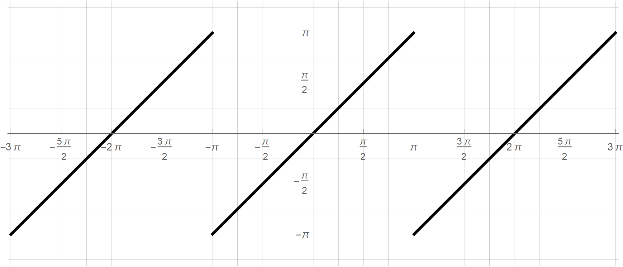
with the following outputPlot[ {Mod[t, 2 Pi, -Pi]}, {t, -3 Pi, 3 Pi}, PlotStyle -> {{RGBColor[0, 0, 0], Thickness[0.005]}}, Ticks -> {Range[-5 Pi, 5 Pi, Pi/2], Range[-5 Pi, 5 Pi, Pi/2]}, PlotRange -> {{-3 Pi - 0.1, 3 Pi + 0.1}, {-Pi - 1, Pi + 1}}, GridLines -> {Range[-5 Pi, 5 Pi, Pi/4], Range[-5 Pi, 5 Pi, Pi/4]}, AspectRatio -> Automatic, ImageSize -> 600 ]
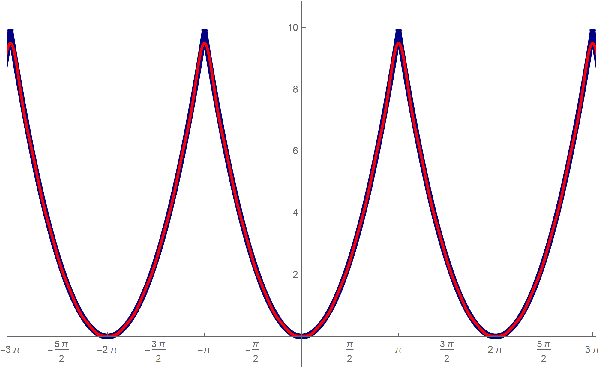
nn = 10;  Plot[
      {Mod[t, 2 Pi, -Pi]^2, \[Pi]^2/3*1 + Sum[(4 (-1)^k)/k^2*Cos[k t], {k, 1, nn}]},
              {t, -4 Pi, 4 Pi}, PlotPoints -> {100, 200},
  PlotStyle -> {{RGBColor[0, 0, 0.5],
     Thickness[0.01]}, {RGBColor[1, 0, 0], Thickness[0.005]}},
  Ticks -> {Range[-4 Pi, 4 Pi, Pi/2], Range[-14, 14, 2]},
  PlotRange -> {{-3 Pi - 0.1, 3 Pi + 0.1}, {-1, Pi^2 + 1}},
  AspectRatio -> Automatic, ImageSize -> 600
        ]
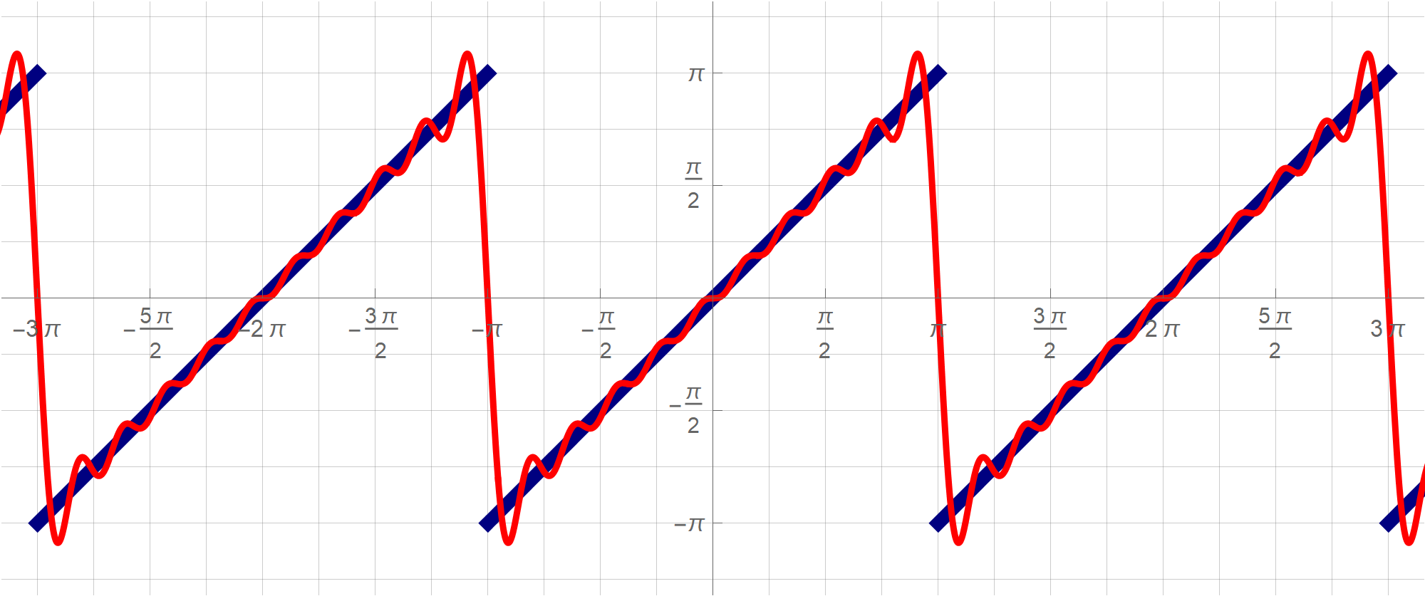
nn = 10;  Plot[
{Mod[t, 2 Pi, -Pi], Sum[-((2 (-1)^k)/k)*Sin[k t], {k, 1, nn}]},
       {t, -4 Pi, 4 Pi}, PlotPoints -> {100, 200},
 PlotStyle -> {{RGBColor[0, 0, 0.5], Thickness[0.01]}, {RGBColor[1, 0, 0], Thickness[0.005]}},
 Ticks -> {Range[-4 Pi, 4 Pi, Pi/2], Range[-4 Pi, 4 Pi, Pi/2]},
 GridLines -> {Range[-4 Pi, 4 Pi, Pi/4], Range[-4 Pi, 4 Pi, Pi/4]},
 PlotRange -> {{-3 Pi - 0.5, 3 Pi + 0.5}, {-Pi - 1, Pi + 1}},
 AspectRatio -> Automatic, ImageSize -> 600
            ]
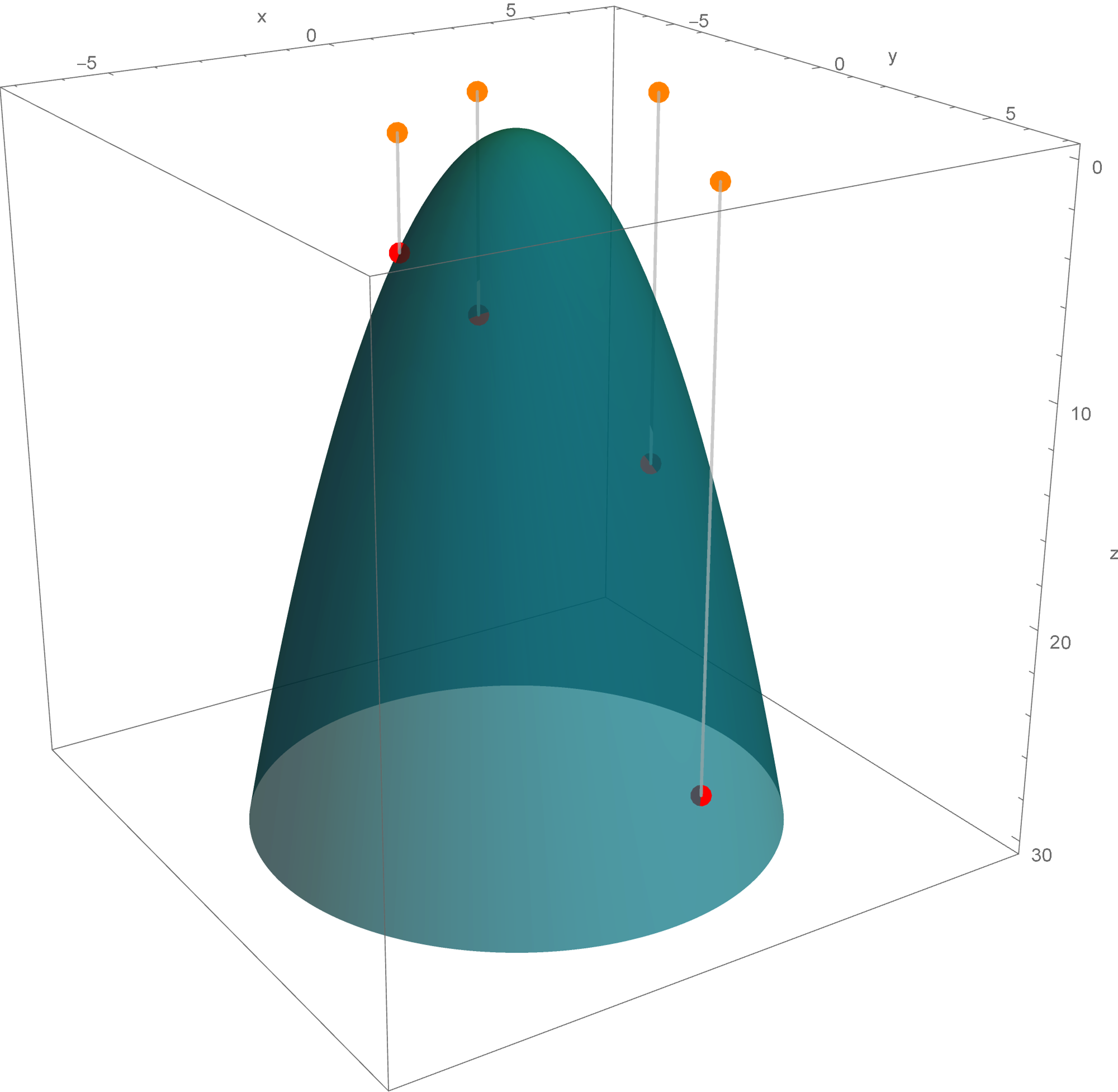
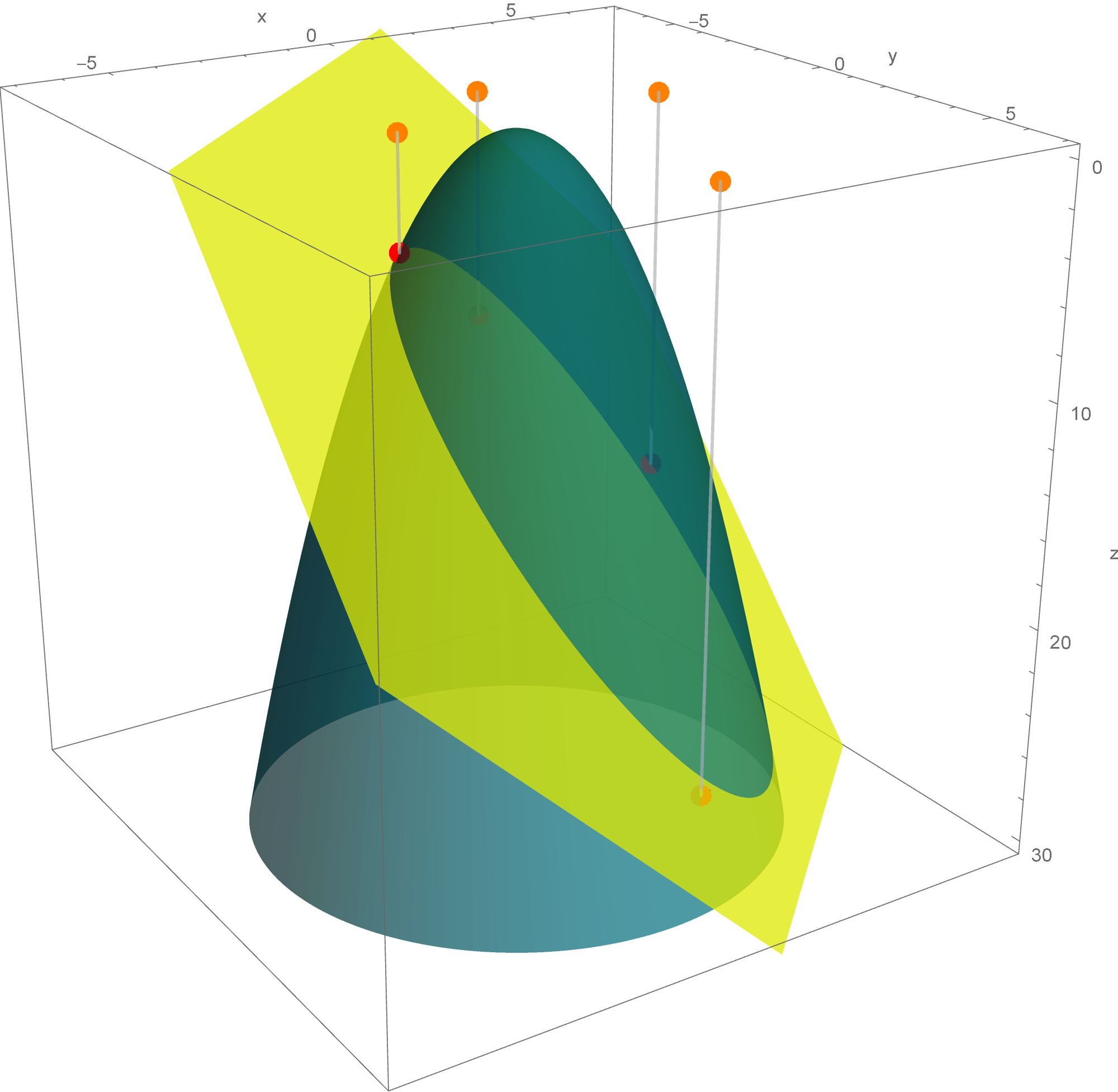
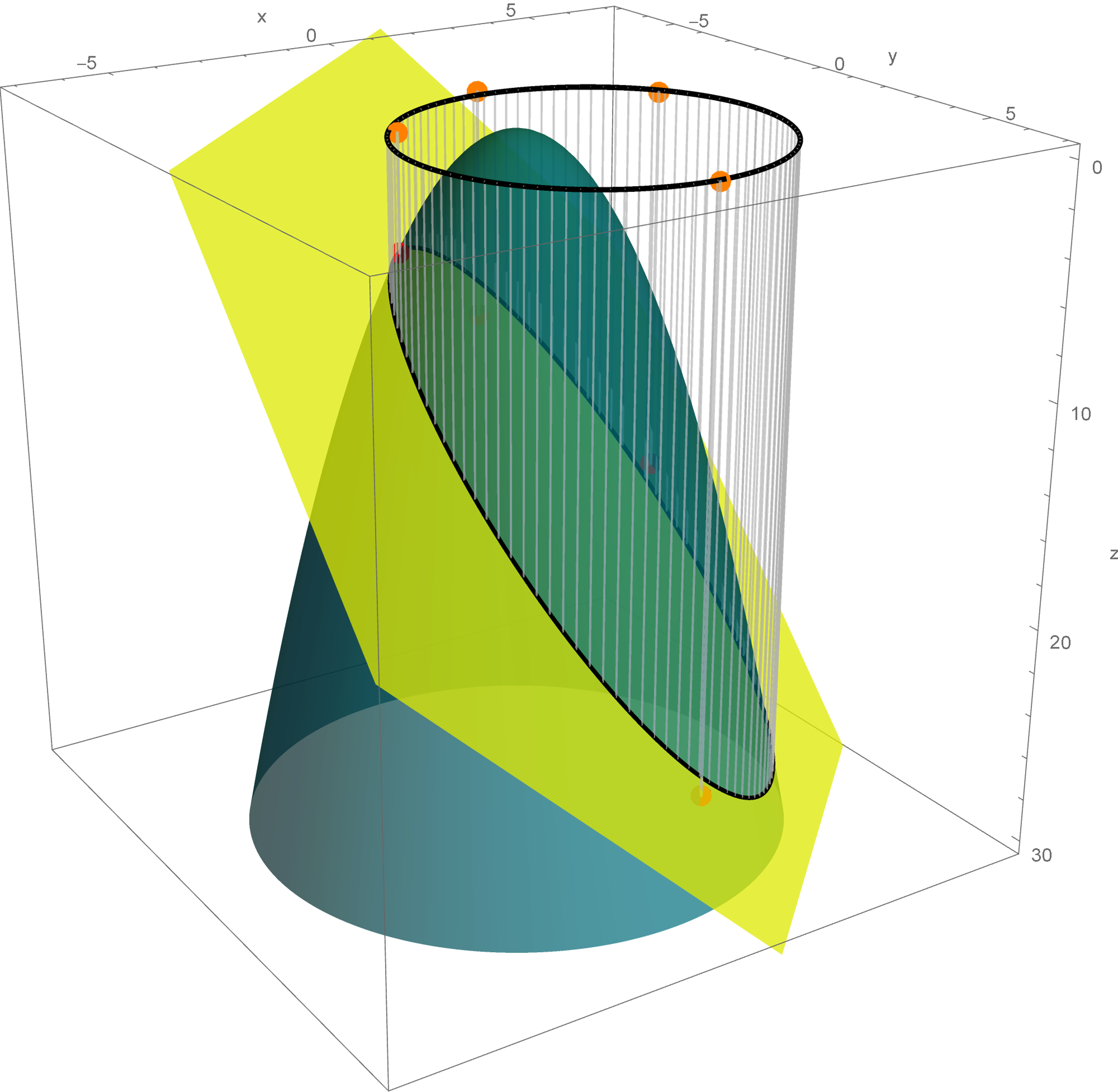
Yesterday we described a method of finding, in a certain way, the best fit circle to a given set of points. The method is identical to finding the least-squares fit plane to a set of given points. In this case all the given points lie on the canonical rotated paraboloid $z = x^2+y^2.$
Let $n$ be a positive integer greater than $2.$ Assume that we are given $n$ noncollinear points in $\mathbb{R}^2$: \[ (x_1, y_1), \ \ (x_2, y_2), \ \ \ldots, \ (x_n, y_n). \]
The normal equations for the system from the preceding item are \[ \left[\begin{array}{cccc} 1 & 1 & \cdots & 1 \\[-3pt] x_1 & x_2 & \cdots & x_n \\ y_1 & y_2 & \cdots & y_n \end{array} \right] \left[\begin{array}{ccc} 1 & x_1 & y_1 \\ 1 & x_2 & y_2 \\ \vdots & \vdots & \vdots \\ 1 & x_n & y_n \end{array} \right] \left[\begin{array}{c} \color{red}{\beta_0} \\ \color{red}{\beta_1} \\ \color{red}{\beta_2} \end{array} \right] = \left[\begin{array}{cccc} 1 & 1 & \cdots & 1 \\[-3pt] x_1 & x_2 & \cdots & x_n \\ y_1 & y_2 & \cdots & y_n \end{array} \right] \left[\begin{array}{c} (x_1)^2 + (y_1)^2 \\ (x_2)^2 + (y_2)^2 \\ \vdots \\ (x_n)^2 + (y_n)^2 \end{array} \right]. \]
You can copy-paste this command to a Mathematica notebook and test it on a set of points. The output of the command is a pair of the best circle's center and the best circle's radius.Clear[BestCir, gpts, mX, vY, abc]; BestCir[gpts_] := Module[ {mX, vY, abc}, mX = Transpose[Append[Transpose[gpts], Array[1 &, Length[gpts]]]]; vY = (#[[1]]^2 + #[[2]]^2) & /@ gpts; abc = Last[ Transpose[ RowReduce[ Transpose[ Append[Transpose[Transpose[mX] . mX], Transpose[mX] . vY] ] ] ] ]; {{abc[[1]]/2, abc[[2]]/2}, Sqrt[abc[[3]] + (abc[[1]]/2)^2 + (abc[[2]]/2)^2]} ]
You can copy-paste the above code in a Mathematica cell and execute it. The result will be the following image:mypts = {{5, 2}, {-1, 5}, {3, -2}, {3, 4.5}, {-5/2, 3}, {1, 5}, {4, 3}, {-3, 1}, {-3/2, 4}, {1, -3}, {-2, -1}, {4, -1}}; cir = N[BestCir[mypts]]; Graphics[{ {PointSize[0.015], RGBColor[1, 0.5, 0], Point[#] & /@ mypts}, {RGBColor[0, 0, 0.5], PointSize[0.015], Point[cir[[1]]], Thickness[0.007], Circle[cir[[1]], cir[[2]]]} }, GridLines -> {Range[-20, 20, 1/2], Range[-20, 20, 1/2]}, GridLinesStyle -> {{GrayLevel[0.75]}, {GrayLevel[0.75]}}, Axes -> True, Ticks -> {Range[-7, 7], Range[-7, 7]}, Frame -> False, PlotRange -> {{-5.75, 5.75}, {-5.75, 5.75}}, ImageSize -> 600]
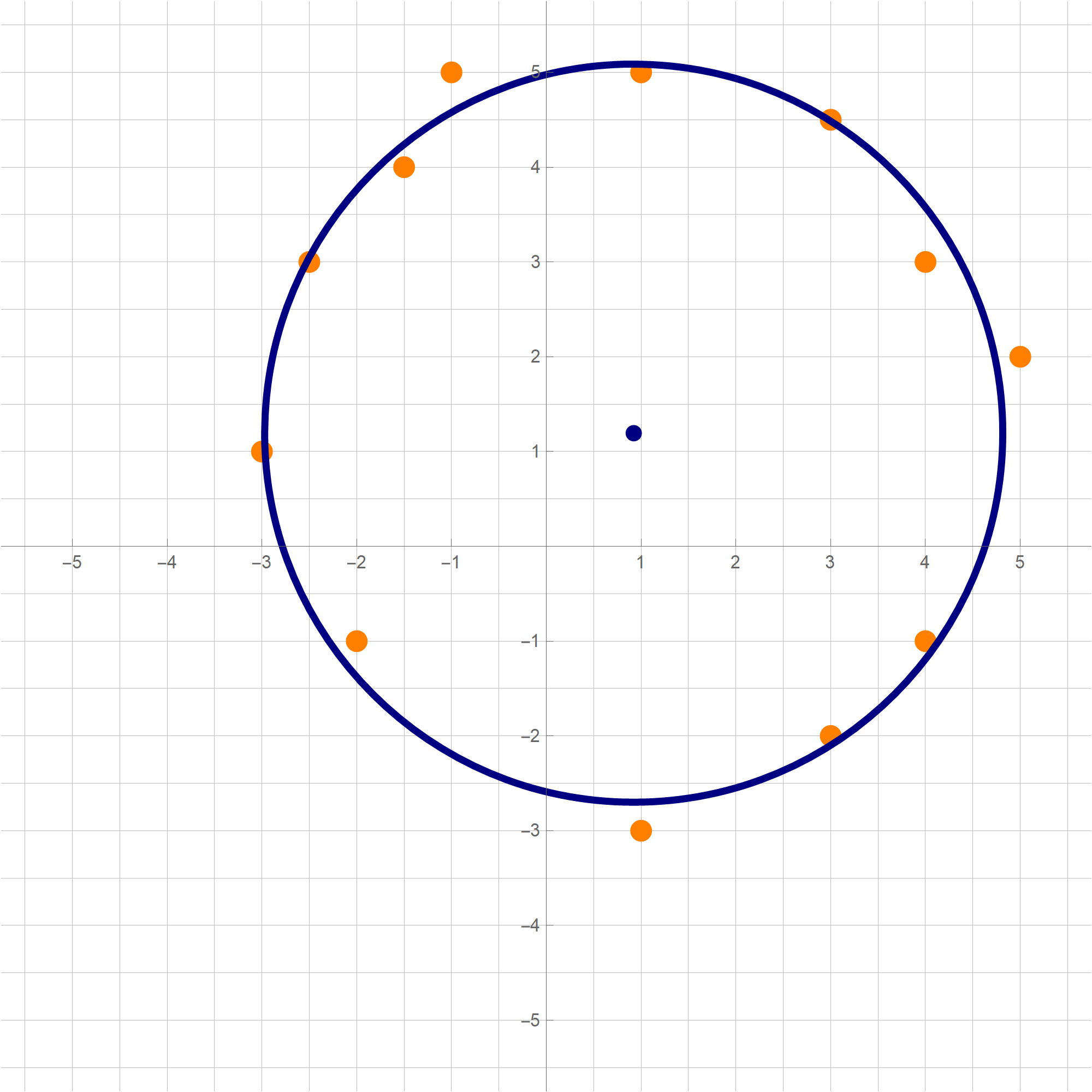
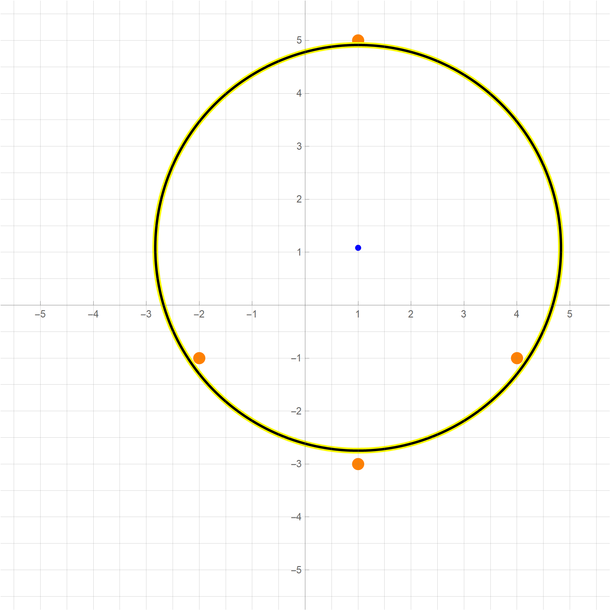
You can copy-paste the above code in a Mathematica cell and execute it. The result will be the following image:mypts = {{3, 1}, {2, -4}, {-2, 3}}; cir = N[BestCir[mypts]]; Graphics[{ {PointSize[0.015], RGBColor[1, 0.5, 0], Point[#] & /@ mypts}, {RGBColor[0, 0, 0.5], PointSize[0.015], Point[cir[[1]]], Thickness[0.007], Circle[cir[[1]], cir[[2]]]} }, GridLines -> {Range[-20, 20, 1/2], Range[-20, 20, 1/2]}, GridLinesStyle -> {{GrayLevel[0.75]}, {GrayLevel[0.75]}}, Axes -> True, Ticks -> {Range[-7, 7], Range[-7, 7]}, Frame -> False, PlotRange -> {{-5.75, 5.75}, {-5.75, 5.75}}, ImageSize -> 600]
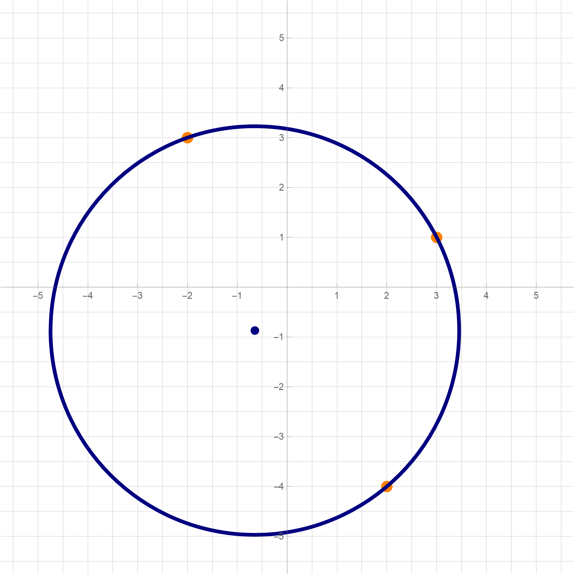
You can copy-paste the above code in a Mathematica cell and execute it. The result will be the following image:mypts = ((4 {Cos[2 Pi #[[1]]], Sin[2 Pi #[[1]]]} + 1/70 {#[[2]], #[[3]]}) & /@ ((RandomReal[#, 3]) & /@ Range[100])); cir = N[BestCir[mypts]]; Graphics[{ {PointSize[0.015], RGBColor[1, 0.5, 0], Point[#] & /@ mypts}, {RGBColor[0, 0, 0.5], PointSize[0.015], Point[cir[[1]]], Thickness[0.007], Circle[cir[[1]], cir[[2]]]} }, GridLines -> {Range[-20, 20, 1/2], Range[-20, 20, 1/2]}, GridLinesStyle -> {{GrayLevel[0.75]}, {GrayLevel[0.75]}}, Axes -> True, Ticks -> {Range[-7, 7], Range[-7, 7]}, Frame -> False, PlotRange -> {{-5.75, 5.75}, {-5.75, 5.75}}, ImageSize -> 600]
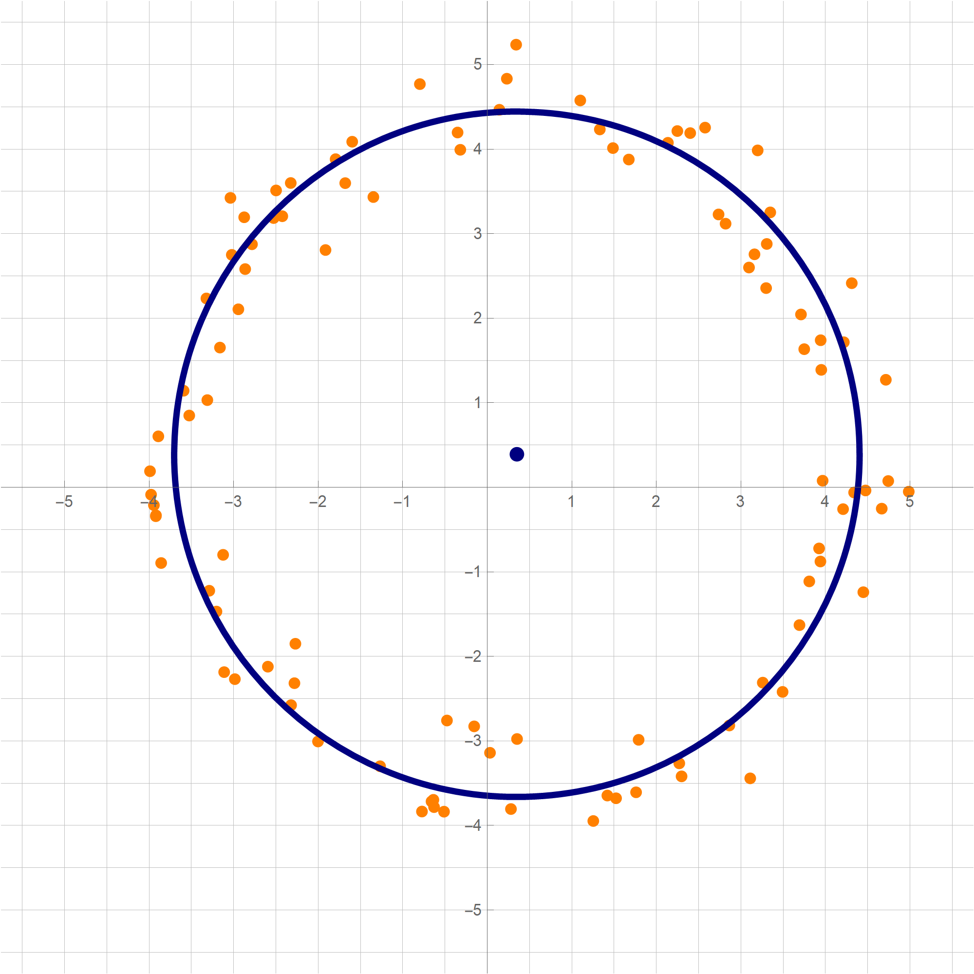
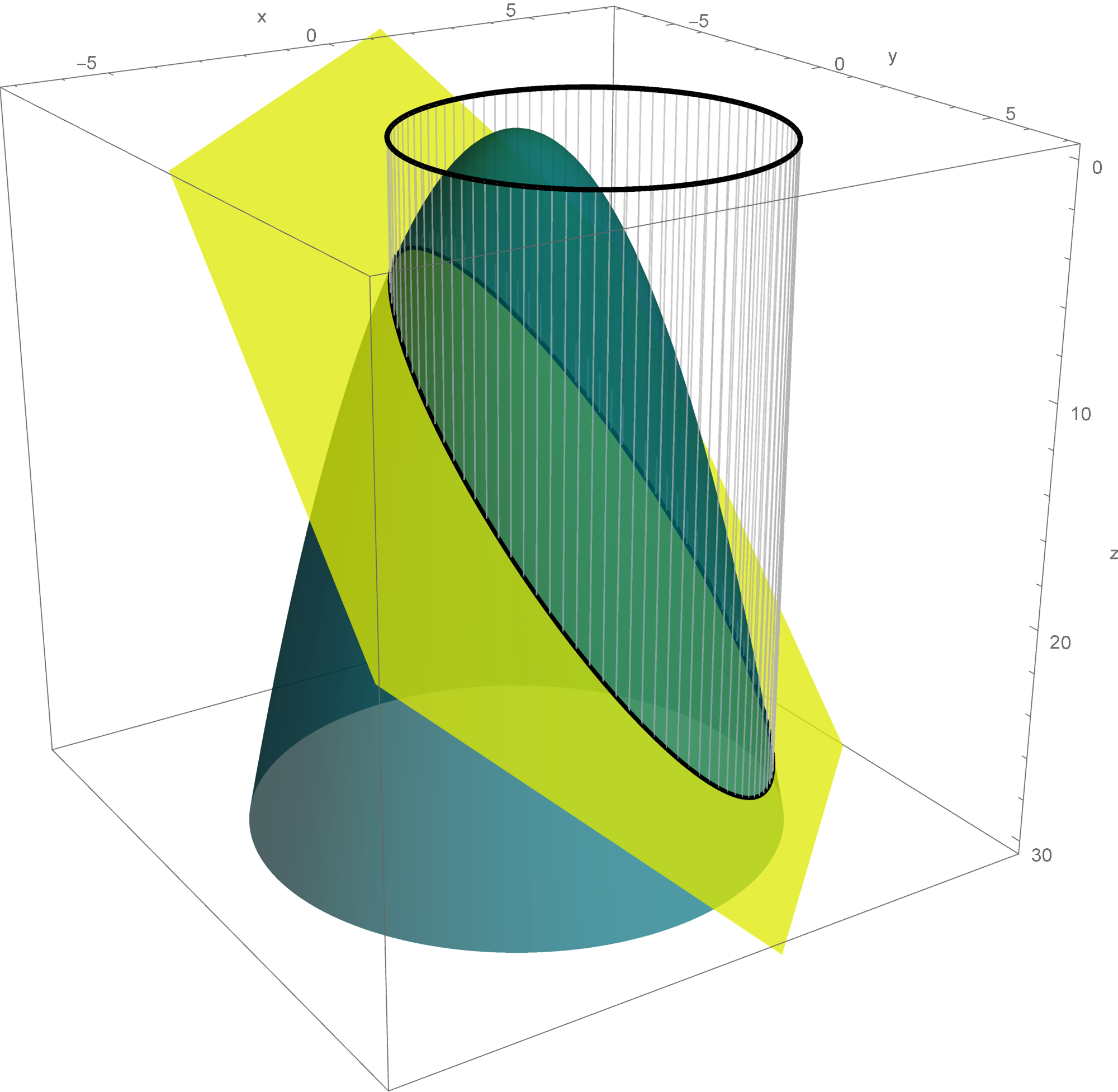
In this item, I recall the definition of an abstract inner product. I implement your suggestions given in class. In the definition below $\times$ denotes the Cartesian product between two sets.
Definition. Let $\mathcal{V}$ be a vector space over $\mathbb R.$ A function \[ \langle\,\cdot\,,\cdot\,\rangle : \mathcal{V}\times\mathcal{V} \to \mathbb{R} \] (this means that for every $u \in \mathcal{V}$ and every $v \in \mathcal{V}$ there exists a unique real number $\langle u,v\rangle \in \mathbb{R}$ which is called the inner product of $u$ and $v$) is called an inner product on $\mathcal{V}$ if it satisfies the following four axioms.
Explanation of the abbreviations: IPC--inner product is commutative, IPA--inner product respects addition, IPS--inner product respects scaling, IPP--inner product is positive definite. The abbreviations are made up by me as cute mnemonic tools.
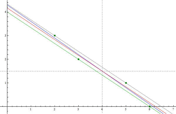
Notice that these four points form a very narrow parallelogram. A characterizing property of a parallelogram is that its diagonals share the midpoint. For this parallelogram, the coordinates of the common midpoint of the diagonals are \[ \overline{x} = \frac{1}{4}(2+3+5+6) = 4, \quad \overline{y} = \frac{1}{4}(3+2+1+0) = 3/2. \] The long sides of this parallelogram are on the parallel lines $y = -2x/3 +4$ and $y = -2x/3 + 13/3.$ It is natural to guess that the least square line is the line which is parallel to these two lines and half-way between them. That is the line $y = -2x/3 + 25/6.$ This line is the red line in the picture below. Clearly this line goes through the point $(4,3/2),$ the intersection of the diagonals of the parallelogram.
The only way to verify this guess is to calculate the least-squares line for these four points. We did that by finding the least-squares solution of the equation \[ \left[\begin{array}{cc} 1 & 2 \\ 1 & 3 \\ 1 & 5 \\ 1 & 6 \end{array} \right] \left[\begin{array}{c} \beta_0 \\ \beta_1 \end{array} \right] = \left[\begin{array}{c} 3 \\ 2 \\ 1 \\ 0 \end{array} \right]. \] To get to the corresponding normal equations we multiply both sides by $X^\top$ \[ \left[\begin{array}{cccc} 1 & 1 & 1 & 1 \\ 2 & 3 & 5 & 6 \end{array} \right] \left[\begin{array}{cc} 1 & 2 \\ 1 & 3 \\ 1 & 5 \\ 1 & 6 \end{array} \right] \left[\begin{array}{c} \beta_0 \\ \beta_1 \end{array} \right] = \left[\begin{array}{cccc} 1 & 1 & 1 & 1 \\ 2 & 3 & 5 & 6 \end{array} \right] \left[\begin{array}{c} 3 \\ 2 \\ 1 \\ 0 \end{array} \right]. \] The corresponding normal equations are \[ \left[\begin{array}{cc} 4 & 16 \\ 16 & 74 \end{array} \right] \left[\begin{array}{c} \beta_0 \\ \beta_1 \end{array} \right] = \left[\begin{array}{c} 6 \\ 17 \end{array} \right]. \] Since the inverse of the above $2\!\times\!2$ matrix is \[ \left[\begin{array}{cc} 4 & 16 \\ 16 & 74 \end{array} \right]^{-1} = \frac{1}{40} \left[\begin{array}{cc} 74 & -16 \\ -16 & 4 \end{array} \right], \] and the solution of the normal equations is unique and it is given by \[ \left[\begin{array}{c} \beta_0 \\ \beta_1 \end{array} \right] = \frac{1}{40} \left[\begin{array}{cc} 74 & -16 \\ -16 & 4 \end{array} \right] \left[\begin{array}{c} 6 \\ 17 \end{array} \right] = \left[\begin{array}{c} \frac{43}{10} \\ -\frac{7}{10} \end{array} \right] \] Hence, the least-squares line for the given data points is \[ y = -\frac{7}{10}x + \frac{43}{10}. \] This line is the blue line in the picture below. The picture below strongly indicates that the blue line also goes through the point $(4,3/2).$ This is easily confirmed: \[ \frac{3}{2} = -\frac{7}{10}4 + \frac{43}{10}. \]
In the image below the forest green points are the given data points. The red line is the line which I guessed could be the least-squares line. The blue line is the true least-squares line.
It is amazing that what we observed in the preceding example is universal. (I proved this fact in class by using completely different method.)
Proposition. If the line $y = \beta_0 + \beta_1 x$ is the least-squares line for the data points \[ (x_1,y_1), \ldots, (x_n,y_n), \] then $\overline{y} = \beta_0 + \beta_1 \overline{x}$, where \[ \overline{x} = \frac{1}{n}(x_1+\cdots+x_n), \quad \overline{y} = \frac{1}{n}(y_1+\dots+y_n). \]
The above proposition is Exercise 14 in Section 6.6.Proof. Let \[ (x_1,y_1), \ldots, (x_n,y_n), \] be given data points and set \[ \overline{x} = \frac{1}{n}(x_1+\cdots+x_n), \quad \overline{y} = \frac{1}{n}(y_1+\dots+y_n). \] Let $y = \beta_0 + \beta_1 x$ be the least-squares line for the given data points. Then the vector $\left[\begin{array}{c} \beta_0 \\ \beta_1 \end{array} \right]$ satisfies the normal equation \[ \left[\begin{array}{cccc} 1 & 1 & \cdots & 1 \\ x_1 & x_2 & \cdots & x_n \end{array} \right] \left[\begin{array}{cc} 1 & x_1 \\ 1 & x_2 \\ \vdots & \vdots \\ 1 & x_n \end{array} \right] \left[\begin{array}{c} \beta_0 \\ \beta_1 \end{array} \right] = \left[\begin{array}{cccc} 1 & 1 & \cdots & 1 \\ x_1 & x_2 & \cdots & x_n \end{array} \right] \left[\begin{array}{c} y_1 \\ y_2 \\ \vdots \\ y_n \end{array} \right]. \] Multiplying the second matrix on the left-hand side and the third vector we get \[ \left[\begin{array}{cccc} 1 & 1 & \cdots & 1 \\ x_1 & x_2 & \cdots & x_n \end{array} \right] \left[\begin{array}{c} \beta_0 + \beta_1 x_1 \\ \beta_0 + \beta_1 x_2 \\ \vdots \\ \beta_0 + \beta_1 x_n \end{array} \right] = \left[\begin{array}{cccc} 1 & 1 & \cdots & 1 \\ x_1 & x_2 & \cdots & x_n \end{array} \right] \left[\begin{array}{c} y_1 \\ y_2 \\ \vdots \\ y_n \end{array} \right]. \] The above equality is an equality of vectors with two components. The top components of these vectors are equal: \[ (\beta_0 + \beta_1 x_1) + (\beta_0 + \beta_1 x_2) + \cdots + (\beta_0 + \beta_1 x_n) = y_1 + y_2 + \cdots + y_n. \] Therefore \[ n \beta_0 + \beta_1 (x_1+x_3 + \cdots + x_n) = y_1 + y_2 + \cdots + y_n. \] Dividing by $n$ we get \[ \beta_0 + \beta_1 \frac{1}{n} (x_1+x_3 + \cdots + x_n) = \frac{1}{n}( y_1 + y_2 + \cdots + y_n). \] Hence \[ \overline{y} = \beta_0 + \beta_1 \overline{x}. \] QED.
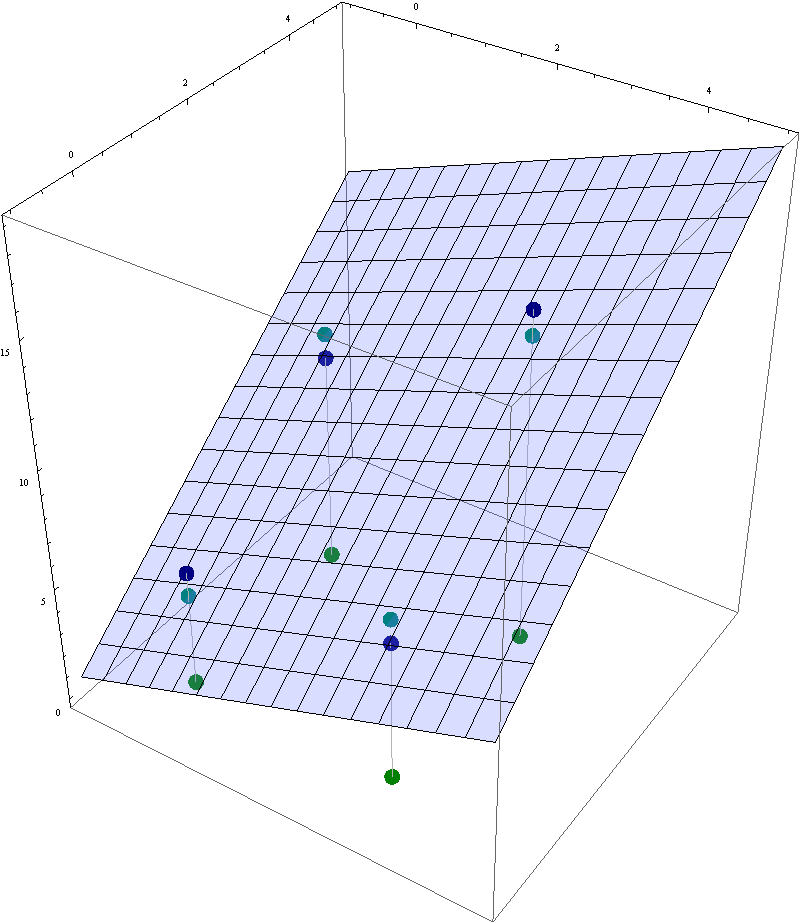
In this image the the navy blue points are the given data points and the light blue plane is the least-squares plane that best fits these data points. The dark green points are their projections onto the $xy$-plane. The teal points are the corresponding points in the least-square plane.
Theorem. Let $A$ be an $n\!\times\!m$ matrix. Then $\operatorname{Nul}(A^\top\!\! A ) = \operatorname{Nul}(A)$.
Proof. The set equality $\operatorname{Nul}(A^\top\!\! A ) = \operatorname{Nul}(A)$ means \[ \mathbf{x} \in \operatorname{Nul}(A^\top\!\! A ) \quad \text{if and only if} \quad \mathbf{x} \in \operatorname{Nul}(A). \] We will prove this equivalence. Assume that $\mathbf{x} \in \operatorname{Nul}(A)$. Then $A\mathbf{x} = \mathbf{0}$. Consequently, \[ (A^\top\!A)\mathbf{x} = A^\top ( \!A\mathbf{x}) = A^\top\mathbf{0} = \mathbf{0}. \] Hence, $(A^\top\!A)\mathbf{x}= \mathbf{0}$, and therefore $\mathbf{x} \in \operatorname{Nul}(A^\top\!\! A )$. Thus, we proved the implication \[ \mathbf{x} \in \operatorname{Nul}(A) \quad \Rightarrow \quad \mathbf{x} \in \operatorname{Nul}(A^\top\!\! A ). \] Now we prove the converse: \[ \tag{*} \mathbf{x} \in \operatorname{Nul}(A^\top\!\! A ) \quad \Rightarrow \quad \mathbf{x} \in \operatorname{Nul}(A). \] Assume, $\mathbf{x} \in \operatorname{Nul}(A^\top\!\! A )$. Then, $(A^\top\!\!A) \mathbf{x} = \mathbf{0}$. Multiplying the last equality by $\mathbf{x}^\top$ we get $\mathbf{x}^\top\! (A^\top\!\! A \mathbf{x}) = 0$. Using the associativity of the matrix multiplication we obtain $(\mathbf{x}^\top\!\! A^\top)A \mathbf{x} = 0$. Using the Linear Algebra with the transpose operation we get $(A \mathbf{x})^\top\!A \mathbf{x} = 0$. Now recall that for every vector $\mathbf{v}$ we have $\mathbf{v}^\top \mathbf{v} = \|\mathbf{v}\|^2$. Thus, we have proved that $\|A\mathbf{x}\|^2 = 0$. Now recall that the only vector whose norm is $0$ is the zero vector, to conclude that $A\mathbf{x} = \mathbf{0}$. This means $\mathbf{x} \in \operatorname{Nul}(A)$. This completes the proof of implication (*). The theorem is proved. □
Corollary 1. Let $A$ be an $n\!\times\!m$ matrix. The columns of $A$ are linearly independent if and only if the $m\!\times\!m$ matrix $A^\top\!\! A$ is invertible.
Corollary 2. Let $A$ be an $n\!\times\!m$ matrix. Then $\operatorname{Col}(A^\top\!\! A ) = \operatorname{Col}(A^\top)$.
Proof 1. The following equalities we established earlier: \begin{align*} \operatorname{Col}(A^\top\!\! A ) & = \operatorname{Row}(A^\top\!\! A ) = \bigl( \operatorname{Nul}(A^\top\!\! A ) \bigr)^\perp, \\ \operatorname{Col}(A^\top) & = \operatorname{Row}(A) = \bigl( \operatorname{Nul}(A) \bigr)^\perp \end{align*} In the above Theorem we proved the following subspaces are equal \[ \operatorname{Nul}(A^\top\!\! A ) = \operatorname{Nul}(A). \] Equal subspaces have equal orthogonal complements: \[ \bigl(\operatorname{Nul}(A^\top\!\! A )\bigr)^\perp = \bigl( \operatorname{Nul}(A) \bigr)^\perp. \] Since earlier we proved \[ \operatorname{Col}(A^\top\!\! A ) = \bigl( \operatorname{Nul}(A^\top\!\! A ) \bigr)^\perp \quad \text{and} \quad \operatorname{Col}(A^\top) = \bigl( \operatorname{Nul}(A) \bigr)^\perp, \] the last three equalities imply \[ \operatorname{Col}(A^\top\!\! A ) = \operatorname{Col}(A^\top). \]
Proof 2. (This is a direct proof. It does not use the above Theorem. It uses the concept of an orthogonal projection.) The set equality $\operatorname{Col}(A^\top\!\! A ) = \operatorname{Col}(A^\top)$ means \[ \mathbf{x} \in \operatorname{Col}(A^\top\!\! A ) \quad \text{if and only if} \quad \mathbf{x} \in \operatorname{Col}(A^\top). \] We will prove this equivalence. Assume that $\mathbf{x} \in \operatorname{Col}(A^\top\!\!A).$ Then there exists $\mathbf{v} \in \mathbb{R}^m$ such that $\mathbf{x} = (A^\top\!\!A)\mathbf{v}.$ Since by the definition of matrix multiplication we have $(A^\top\!\!A)\mathbf{v} = A^\top\!(A\mathbf{v})$, we have $\mathbf{x} = A^\top\!(A\mathbf{v}).$ Consequently, $\mathbf{x} \in \operatorname{Col}(A^\top).$ Thus, we proved the implication \[ \mathbf{x} \in \operatorname{Col}(A^\top\!\!A) \quad \Rightarrow \quad \mathbf{x} \in \operatorname{Col}(A^\top). \] Now we prove the converse: \[ \mathbf{x} \in \operatorname{Col}(A^\top) \quad \Rightarrow \quad \mathbf{x} \in \operatorname{Col}(A^\top\!\!A). \] Assume, $\mathbf{x} \in \operatorname{Col}(A^\top).$ Let $\mathbf{y} \in \mathbb{R}^n$ be such that $\mathbf{x} = A^\top\!\mathbf{y}.$ Let $\widehat{\mathbf{y}}$ be the orthogonal projection of $\mathbf{y}$ onto $\operatorname{Col}(A).$ That is $\widehat{\mathbf{y}} \in \operatorname{Col}(A)$ and $\mathbf{y} - \widehat{\mathbf{y}} \in \bigl(\operatorname{Col}(A)\bigr)^{\perp}.$ Since $\widehat{\mathbf{y}} \in \operatorname{Col}(A),$ there exists $\mathbf{v} \in \mathbb{R}^m$ such that $\widehat{\mathbf{y}} = A\mathbf{v}.$ Since $\bigl(\operatorname{Col}(A)\bigr)^{\perp} = \operatorname{Nul}(A^\top),$ the relationship $\mathbf{y} - \widehat{\mathbf{y}} \in \bigl(\operatorname{Col}(A)\bigr)^{\perp}$ yields $A^\top\bigl(\mathbf{y} - \widehat{\mathbf{y}}\bigr) = \mathbf{0}.$ Consequently, since $\widehat{\mathbf{y}} = A\mathbf{v},$ we deduce $A^\top\bigl(\mathbf{y} - A\mathbf{v}\bigr) = \mathbf{0}.$ Hence \[ \mathbf{x} = A^\top\mathbf{y} = \bigl(A^\top\!\!A\bigr) \mathbf{v} \quad \text{with} \quad \mathbf{v} \in \mathbb{R}^m. \] This proves that $\mathbf{x} \in \operatorname{Col}(A^\top\!\!A).$ Thus, the implication \[ \mathbf{x} \in \operatorname{Col}(A^\top) \quad \Rightarrow \quad \mathbf{x} \in \operatorname{Col}(A^\top\!\!A) \] is proved. The corollary is proved. □
Corollary 3. Let $A$ be an $n\!\times\!m$ matrix. The matrices $A^\top$ and $A^\top\!\! A$ have the same rank.
The cumulative effect of time spent engaged in creative
pursuits is an amazing, often neglected aspect of life.
The school exists for us to engage in creative pursuits and experience the resulting amazing cumulative effect.
Your homework is your creative pursuit. While doing homework, you can use anything that enriches your creative experience. And please notice that in the preceding two sentences, I used the pronoun "you" four times. It is all about you.
Now about me. I will not pretend that I know what is best for you. I am trying to create a mathematical environment where you will be encouraged to engage in creative mathematical pursuits. I am open to all your mathematical questions. I want to hear about your mathematical experiences. I hope to contribute constructively to making that experience more conducive to your mathematical growth.
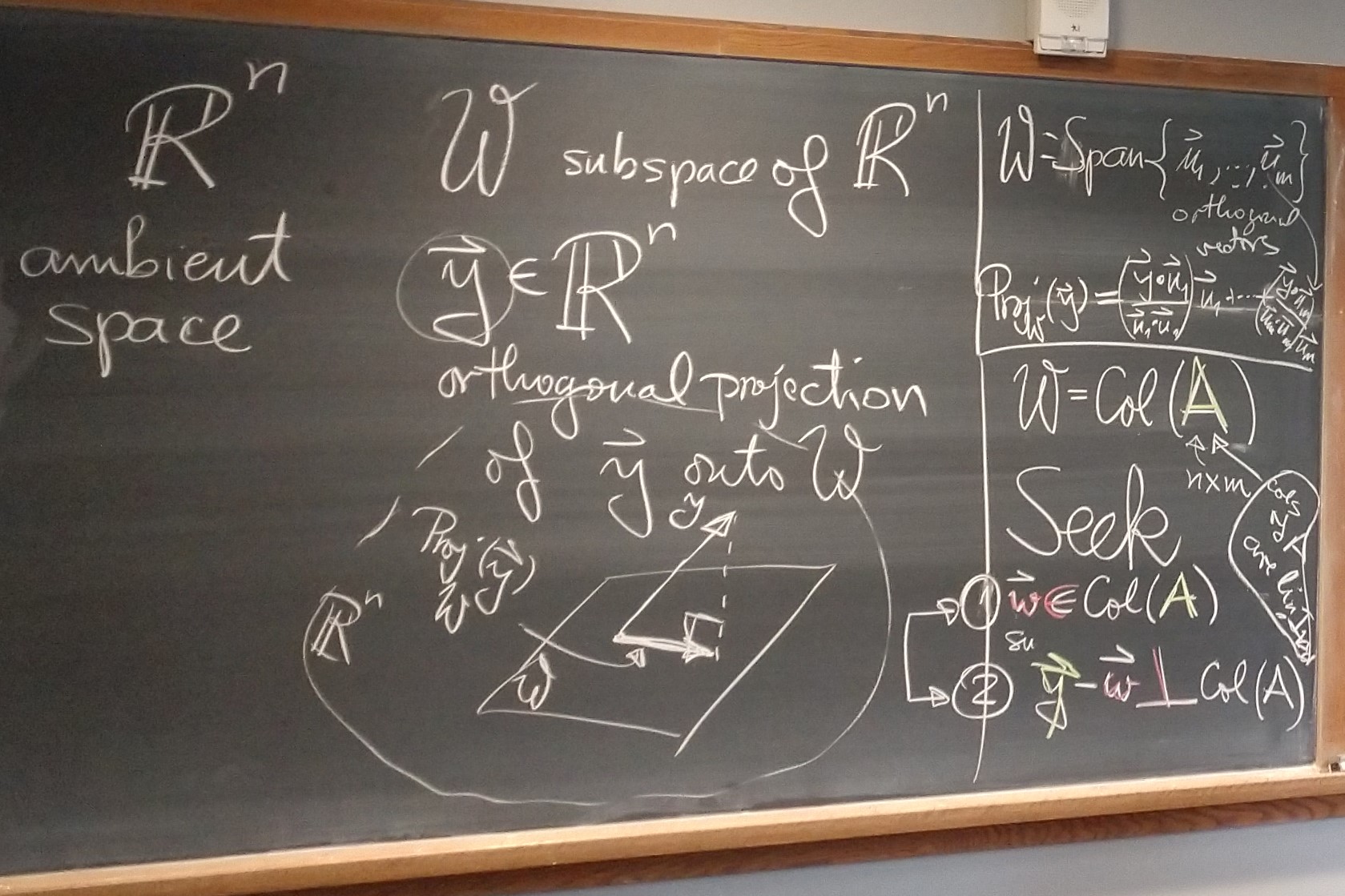
The next question is: How do we calculate the orthogonal projection of $\mathbf{y} \in \mathbb{R}^n$ onto a subspace $\mathcal{W}$ of $\mathbb{R}^n?$
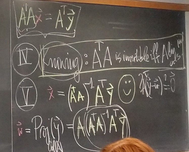
The answer to this question depends on the way how subspace $\mathcal{W}$ is defined. We will consider two casesIn this item I will deduce a formula for $\operatorname{Proj}_{\mathcal W}(\mathbf{y})$ where $\mathbf{y} \in \mathbb{R}^n$ and $\mathcal{W} = \operatorname{Col}(A)$ where $A$ is an $n\!\times\!m$ matrix with linearly independent columns.
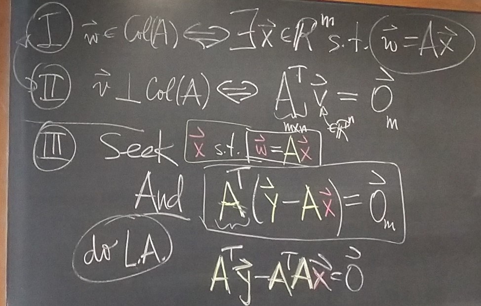
Next, recall our background knowledge about $\operatorname{Col}(\color{green}{A})$ and $\bigl(\operatorname{Col}(\color{green}{A})\bigr)^\perp.$
Our background knowledge about about $\operatorname{Col}(\color{green}{A})$ is: \[ \mathbf{b} \in \operatorname{Col}({A}) \qquad \text{if and only if} \qquad \exists\, \mathbf{x} \in \mathbb{R}^m \ \ \text{such that} \ \ \mathbf{b} = A \mathbf{x}. \]
Our background knowledge about about $\bigl(\operatorname{Col}(\color{green}{A})\bigr)^\perp$ is: \[ \bigl(\operatorname{Col}({A})\bigr)^\perp = \operatorname{Nul}\bigl(A^\top\bigr). \]


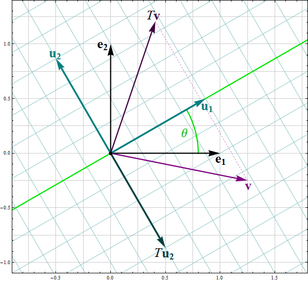
An illustration of a Reflection across the green line
| Equation 1 | Equation 2 | Equation 3 |
|---|---|---|
| \[ \left[\! \begin{array}{rr} 1 & -4 \\ -3 & 1 \\ 1 & 2 \end{array} \!\right] \left[\! \begin{array}{c} x_1 \\ x_2 \end{array} \!\right] = \left[\! \begin{array}{r} 2 \\ 1 \\ -4 \end{array} \!\right] \] | \[ \left[\! \begin{array}{rr} 1 & -4 \\ -3 & 1 \\ 1 & 2 \end{array} \!\right] \left[\! \begin{array}{c} x_1 \\ x_2 \end{array} \!\right] = \left[\!\begin{array}{r} 6 \\ -7 \\ 0\end{array}\! \right] \] | \[ \left[\! \begin{array}{rr} 1 & -4 \\ -3 & 1 \\ 1 & 2 \end{array} \!\right] \left[\! \begin{array}{c} x_1 \\ x_2 \end{array} \!\right] = \left[\!\begin{array}{r} -7 \\ -1 \\ 5\end{array} \!\right] \] |
(n-by-n matrix M) (k-th column of the n-by-n identity matrix) = (k-th column of the n-by-n matrix M).
Place the cursor over the image to start the animation.
|
|
|
|
|
|
|
|
|
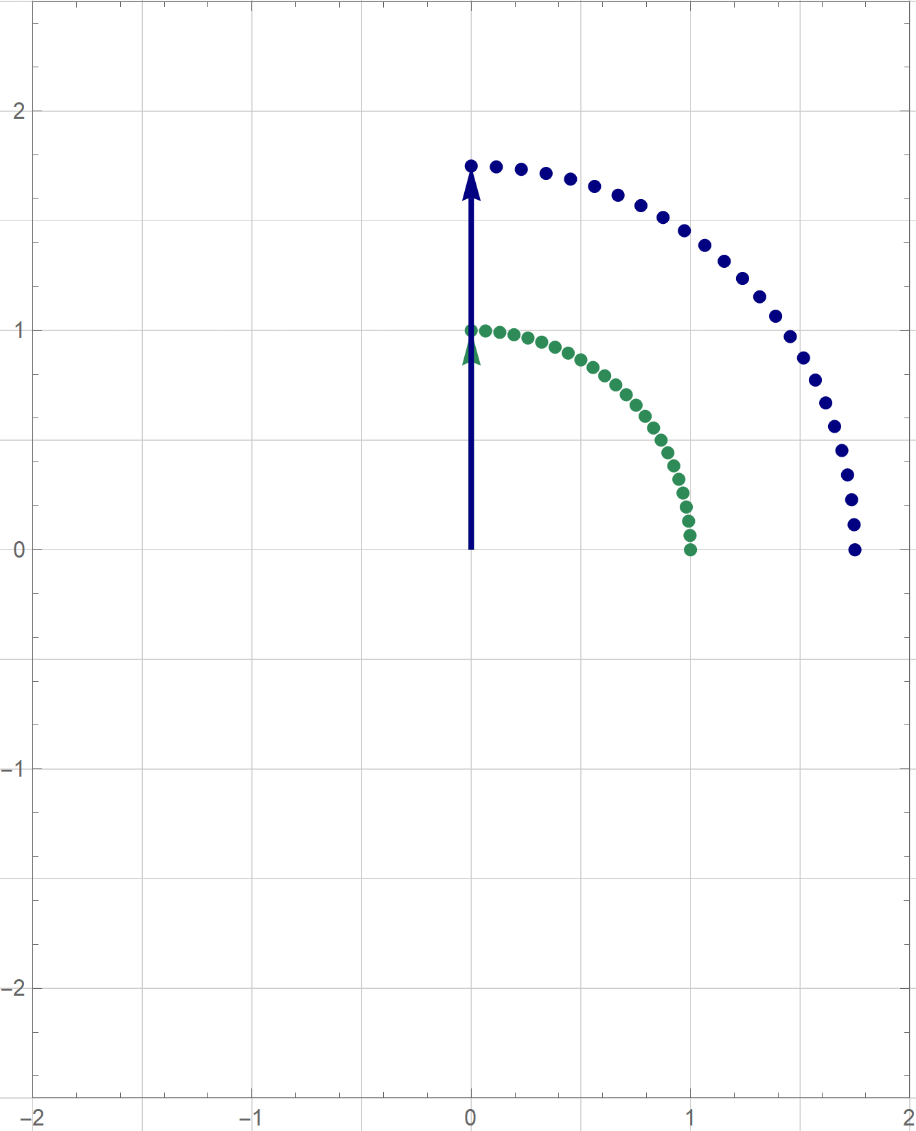
|
The preceding formula gives $\cos(nt)$ expressed in terms of two previous multiple angle cosines $\cos\bigl((n-1)t \bigr)$ and $\cos\bigl((n-2)t \bigr).$ Such a formula is called a recursion or a recurrence relation.
The most famous recursion is the formula for the Fibonacci numbers. That formula gives the next number based on the previous two.
Here is a proof.
We prove that the only linear combination of the functions $\mathbf{a}_0, \mathbf{a}_1, \mathbf{a}_2, \mathbf{a}_3,\mathbf{a}_4, \mathbf{a}_5, \mathbf{a}_{6}$ which results in the zero function is the trivial linear combination.
|
${\mathbf{b}}_0 = 1$ |
${\mathbf{a}}_0 = 1$ |
|
${\mathbf{b}}_1 = \cos t$ |
${\mathbf{a}}_1 = \cos t$ |
|
${\mathbf{b}}_2 = \cos(2t)$ |
${\mathbf{a}}_2 = (\cos t)^2$ |
|
${\mathbf{b}}_3 = \cos(3t)$ |
${\mathbf{a}}_3 = (\cos t)^3$ |
|
${\mathbf{b}}_4 = \cos(4t)$ |
${\mathbf{a}}_4 = (\cos t)^4$ |
|
${\mathbf{b}}_5 = \cos(5t)$ |
${\mathbf{a}}_5 = (\cos t)^5$ |
|
${\mathbf{b}}_6 = \cos(6t)$ |
${\mathbf{a}}_6 = (\cos t)^6$ |
|
$(\cos t)^6 \approx \frac{5}{16}$ |
|
$(\cos t)^6 \approx \frac{5}{16}+\frac{15}{32} \cos(2t)$ |
|
$(\cos t)^6 \approx \frac{5}{16}+\frac{15}{32} \cos(2t)+\frac{3}{16} \cos(4t)$ |
|
$(\cos t)^6 = \frac{5}{16}+\frac{15}{32} \cos(2t)+\frac{3}{16} \cos(4t)+\frac{1}{32} \cos(6t)$ |
How to convert the definition from the preceding item into something tangible? Since the statement of the definition includes for all vectors $\mathbf{v}\in \mathcal{H}$, a natural strategy is to look for some friendly vectors in $\mathcal{H}$ and assess what the definition tells us for those friendly vectors. In this context, the friendly vectors are vectors in the basis $\mathcal{A} = \bigl\{\mathbf{a}_1,\ldots,\mathbf{a}_m\bigr\}$ and the basis $\mathcal{B} = \bigl\{\mathbf{b}_1,\ldots,\mathbf{b}_m\bigr\}.$
So, what does the definition of the change of coordinates matrix tells us about the vectors in the basis $\mathcal{A} = \bigl\{\mathbf{a}_1,\ldots,\mathbf{a}_m\bigr\}?$ It tells the following \[ \underset{\mathcal{B}\leftarrow\mathcal{A}}{P} \bigl[\mathbf{a}_k\bigr]_\mathcal{A} = \bigl[\mathbf{a}_k\bigr]_\mathcal{B} \quad \text{for all} \quad k \in \{1,\ldots,m\}. \] Is this informative? Do you know what the vectors \[ \bigl[\mathbf{a}_1\bigr]_\mathcal{A}, \ \bigl[\mathbf{a}_2\bigr]_\mathcal{A}, \ldots , \bigl[\mathbf{a}_m\bigr]_\mathcal{A} \] are? The simplest answer to this question is to put these vectors in an $m\!\times\!m$ matrix. What is that matrix? Here is the answer: \[ \Bigl[ \bigl[\mathbf{a}_1\bigr]_{\mathcal{A}} \ \cdots \ \bigl[ \mathbf{a}_m\bigr]_{\mathcal{A}} \Bigr] = I_m. \] That is, the vectors $\bigl[\mathbf{a}_1\bigr]_\mathcal{A}, \ldots , \bigl[\mathbf{a}_m\bigr]_\mathcal{A}$ are the columns of the identity matrix $I_m.$ Next, we calculate \begin{align*} \underset{\mathcal{B}\leftarrow\mathcal{A}}{P} & = \left(\underset{\mathcal{B}\leftarrow\mathcal{A}}{P}\right) I_m \\ & = \left(\underset{\mathcal{B}\leftarrow\mathcal{A}}{P}\right) \Bigl[ \bigl[\mathbf{a}_1\bigr]_{\mathcal{A}} \ \cdots \ \bigl[ \mathbf{a}_m\bigr]_{\mathcal{A}} \Bigr] \\ & = \Bigl[ \underset{\mathcal{B}\leftarrow\mathcal{A}}{P} \bigl[\mathbf{a}_1\bigr]_{\mathcal{A}} \ \cdots \ \underset{\mathcal{B}\leftarrow\mathcal{A}}{P} \bigl[ \mathbf{a}_m\bigr]_{\mathcal{A}} \Bigr] \\ & = \Bigl[ \bigl[\mathbf{a}_1\bigr]_{\mathcal{B}} \ \cdots \ \bigl[ \mathbf{a}_m\bigr]_{\mathcal{B}} \Bigr] \end{align*}
Finally, we have something that we can calculate: \[ \underset{\mathcal{B}\leftarrow\mathcal{A}}{P} = \Bigl[ \bigl[\mathbf{a}_1\bigr]_{\mathcal{B}} \ \cdots \ \bigl[ \mathbf{a}_m\bigr]_{\mathcal{B}} \Bigr]. \]Below is a proof that the monomials $1, x, x^2, x^3$ are linearly independent in the vector space ${\mathbb P}_3$. First we need to be specific what we need to prove.
Let $\alpha_1,$ $\alpha_2,$ $\alpha_3,$ and $\alpha_4$ be scalars in $\mathbb{R}.$ We need to prove the following implication: If \[ \require{bbox} \bbox[5px, #88FF88, border: 1pt solid green]{\alpha_1\cdot 1 + \alpha_2 x + \alpha_3 x^2 + \alpha_4 x^3 =0 \quad \text{for all} \quad x \in \mathbb{R}}, \] then \[ \bbox[5px, #FF4444, border: 1pt solid red]{\alpha_1 = 0, \quad \alpha_2 =0, \quad \alpha_3 = 0, \quad \alpha_4 = 0}. \] Proof.
Definition. A function $f$ from $A$ to $B$, $f:A\to B$, is called surjection if it satisfies condition the following condition:
Definition. A function $f$ from $A$ to $B$, $f:A\to B$, is called injection if it satisfies the following condition
An equivalent formulation of the preceding condition is:
Definition. A function $f:A\to B$ is called bijection if it it satisfies the following two conditions:
In other words, a function $f:A\to B$ is called bijection if it is both an injection and a surjection.
Definition. Let $\mathcal V$ and $\mathcal W$ be vector spaces. A linear bijection $T: \mathcal V \to \mathcal W$ is said to be an isomorphism.
Theorem 8. Let $n \in \mathbb{N}$. Let $\mathcal{B} = \{\mathbf{b}_1, \ldots, \mathbf{b}_n\}$ be a basis of a vector space $\mathcal V$. The coordinate mapping \[ \mathbf{v} \mapsto [\mathbf{v}]_\mathcal{B}, \qquad \mathbf{v} \in \mathcal V, \] is a linear bijection between the vector space $\mathcal V$ and the vector space $\mathbb{R}^n.$
Theorem 8. Let $n \in \mathbb{N}$. Let $\mathcal{B} = \{\mathbf{b}_1, \ldots, \mathbf{b}_n\}$ be a basis of a vector space $\mathcal V$. The coordinate mapping \[ \mathbf{v} \mapsto [\mathbf{v}]_\mathcal{B}, \qquad \mathbf{v} \in \mathcal{V}, \] is an isomorphism between the vector space $\mathcal V$ and the vector space $\mathbb{R}^n.$
Corollary 1. Let $m, n \in \mathbb{N}$. Let $\mathcal{B} = \{\mathbf{b}_1, \ldots, \mathbf{b}_n\}$ be a basis of a vector space $\mathcal V$. Then the following statements are equivalent:
Corollary 2. Let $m, n \in \mathbb{N}$. Let $\mathcal{B} = \{\mathbf{b}_1, \ldots, \mathbf{b}_n\}$ be a basis of a vector space $\mathcal V$. Then the following statements are equivalent:
Problem. Denote by $\mathcal{V}$ the vector space of all continuous real valued functions defined on $\mathbb{R},$ see Example 5 on page 194, Section 4.1, in the textbook. Consider the following subset of $\mathcal{V}:$ \[ \mathcal{S}_1 := \Big\{ f \in \mathcal{V} : \exists \ a, b \in \mathbb{R} \ \ \text{such that} \ \ f(x) = a \sin(x+b) \ \ \forall x\in\mathbb{R} \Big\} . \] Prove that $\mathcal{S}_1$ is a subspace of $\mathcal{V}$ and determine its dimension.
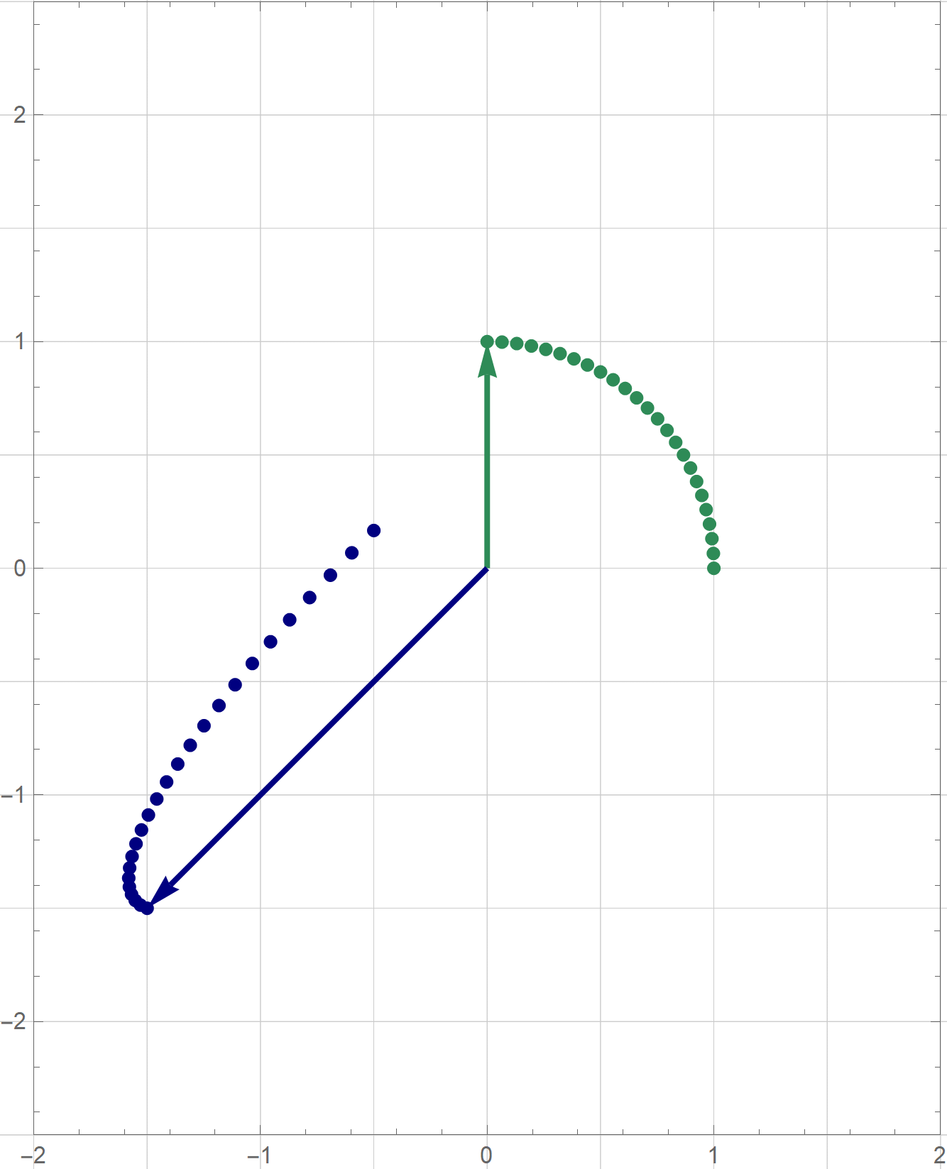
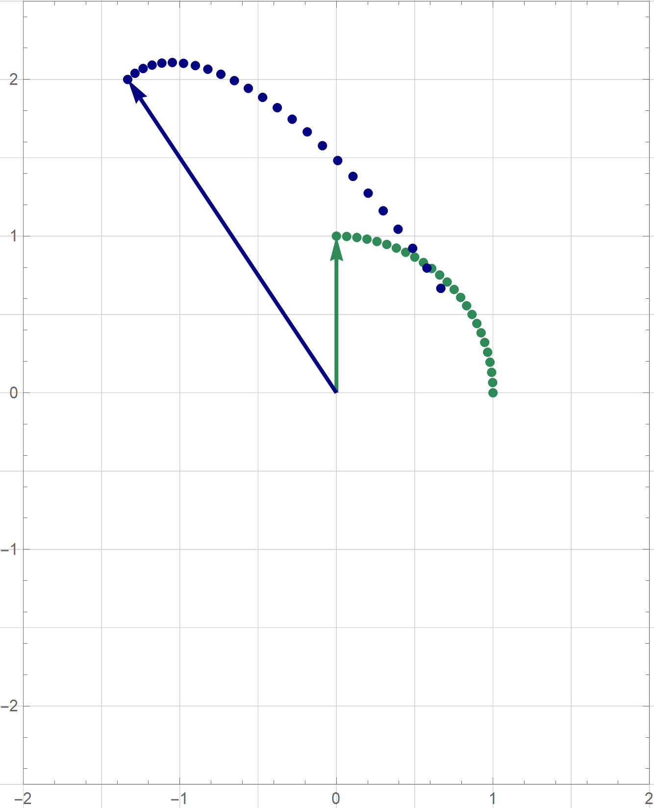
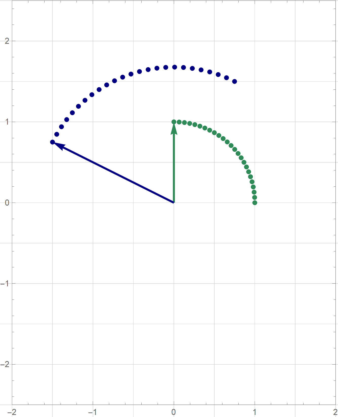
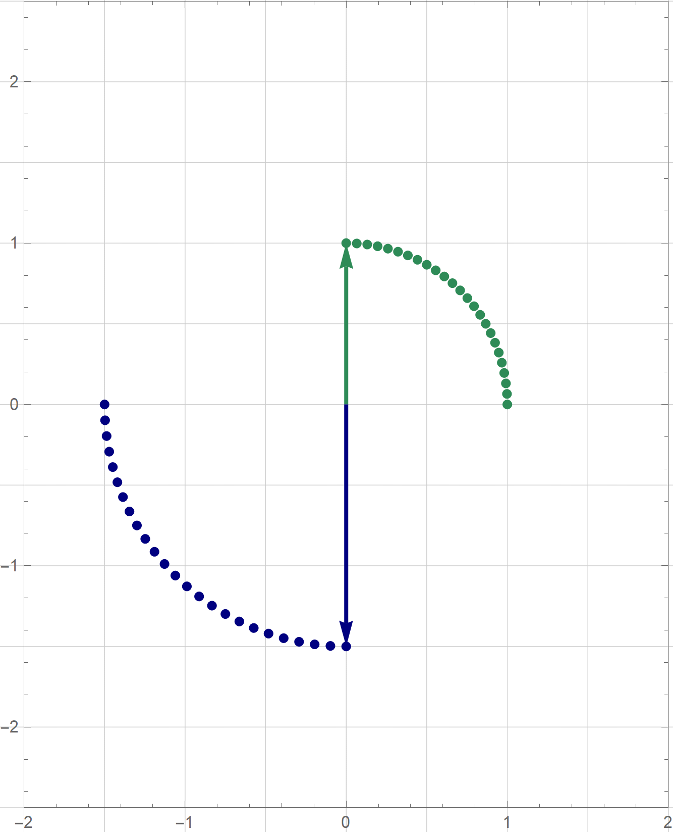
The first step towards a solution of this problem would be to familiarize ourselves with the set $\mathcal{S}_1.$ Which functions are in $\mathcal{S}_1?$ For example, with $a=1$ and $b=0$, the function $\sin(x)$ is in the set $\mathcal{S}_1,$ with $a=1$ and $b=\pi/2$, the function $\sin(x+\pi/2) = \cos(x)$ is in the set $\mathcal{S}_1.$ This is a big discovery: the functions $\sin(x)$ and $\cos(x)$ are both in the set $\mathcal{S}_1.$
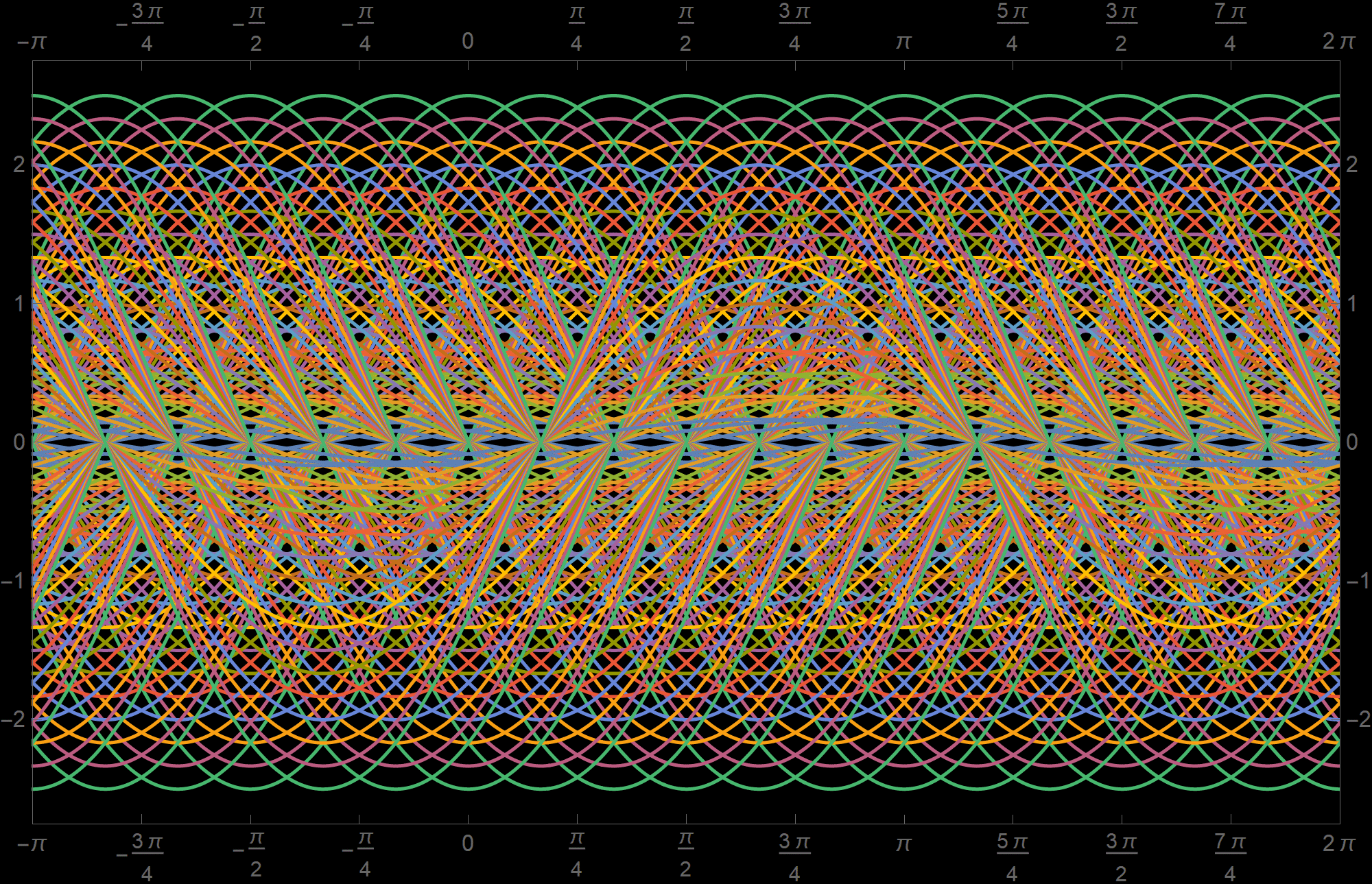
Below I present 180 functions from $\mathcal{S}_1$ with the coefficients \[ a \in \left\{\frac{1}{6}, \frac{1}{3}, \frac{1}{2}, \frac{2}{3}, \frac{5}{6}, 1, \frac{7}{6}, \frac{4}{3}, \frac{3}{2}, \frac{5}{3}, \frac{11}{6},2, \frac{13}{6}, \frac{7}{3}, \frac{5}{2} \right\}\quad \text{and} \quad b \in \left\{ 0, \frac{\pi}{6},\frac{\pi}{3},\frac{\pi}{2},\frac{2\pi}{3}, \frac{5\pi}{6}, \pi, \frac{7\pi}{6},\frac{4\pi}{3},\frac{3\pi}{2},\frac{5\pi}{3}, \frac{11\pi}{6} \right\} \]
Place the cursor over the image to see individual functions.
It is useful to recall the trigonometric identity called the angle sum identity for the sine function: For arbitrary real numbers $x$ and $y$ we have \[ \sin(x + y) = (\sin x) (\cos y) + (\cos x)(\sin y). \]
Applying the above angle sum identity to $\sin(x+b)$ we get \[ \sin(x + b) = (\sin x) (\cos b) + (\cos x)(\sin b) = (\cos b) (\sin x) + (\sin b) (\cos x). \] Consequently, for an arbitrary function $f(x) = a \sin(x+b)$ from $\mathcal{S}_1$ we have \[ f(x) = a \sin(x+b) = a (\cos b) (\sin x) + a (\sin b) (\cos x) \qquad \text{for all} \quad x \in \mathbb{R}. \] The last formula tells us that for given numbers $a$ and $b$ the function $a \sin(x+b)$ is a linear combination of the functions $\sin x$ and $\cos x$. And this is true for each function in $\mathcal{S}_1$: each function in $\mathcal{S}_1$ is a linear combination of $\sin x$ and $\cos x$.
Since each function in $\mathcal{S}_1$ is a linear combination of $\sin x$ and $\cos x$, we have proved that \[ \mathcal{S}_1 \subseteq \operatorname{Span}\bigl\{\sin x, \cos x \bigr\}. \]
The inclusion that we proved in the preceding item inspires us to claim that the converse inclusion holds as well. We claim that \[ \operatorname{Span}\bigl\{\sin x, \cos x \bigr\} \subseteq \mathcal{S}_1. \] That is, we claim that each linear combination of $\sin x$ and $\cos x$ belongs to the set $\mathcal{S}_1.$
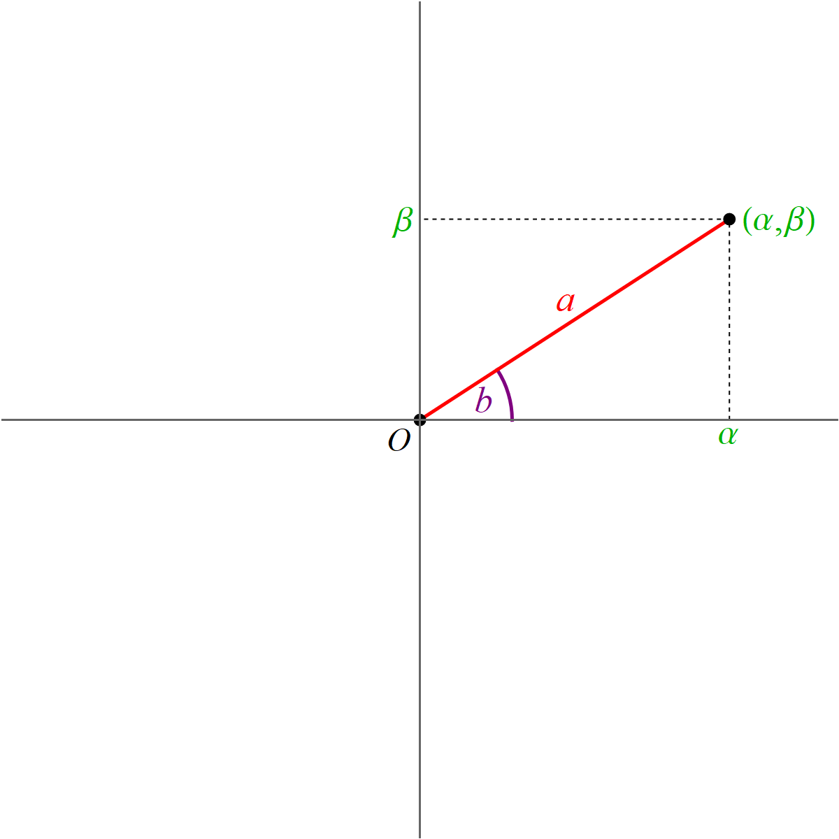
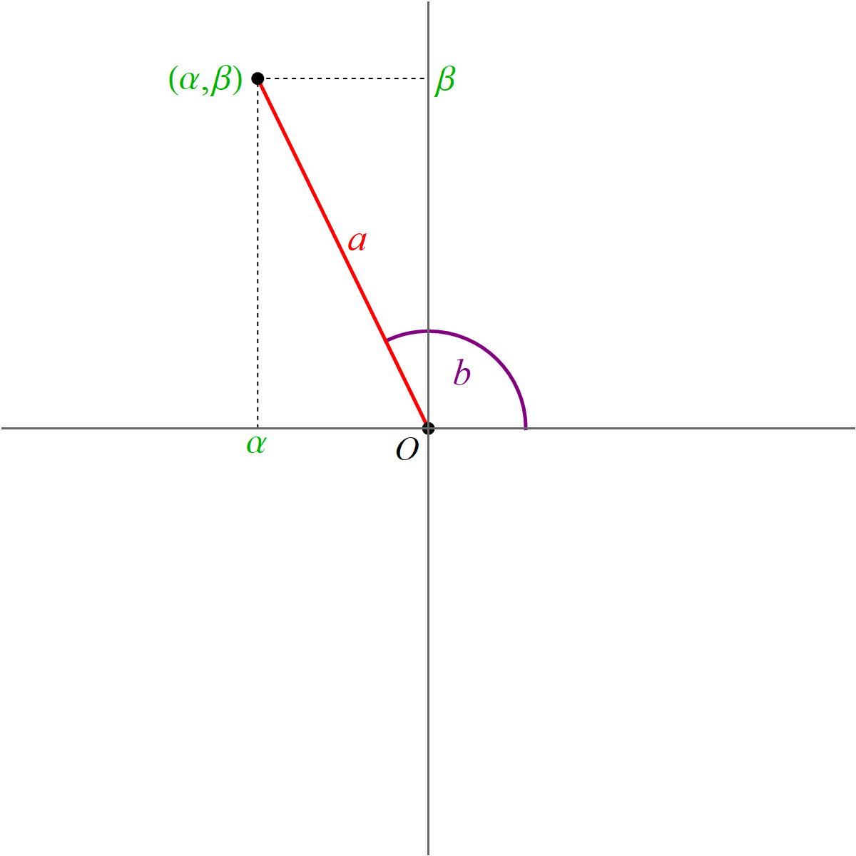
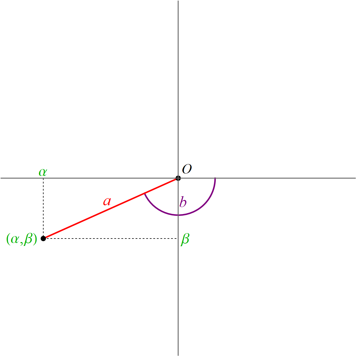
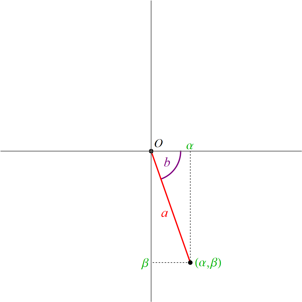
To prove the claim stated in the preceding item we need to formulate that claim using numbers. We take an arbitrary linear combination of $\sin x$ and $\cos x$. That is we take arbitrary real numbers $\alpha$ and $\beta$ and consider the linear combination \[ \alpha (\sin x) + \beta (\cos x). \] We need to prove that there exist real numbers $a$ and $b$ such that \[ \alpha (\sin x) + \beta (\cos x) = a \sin(x+b) \qquad \text{for all} \quad x \in \mathbb{R}. \] In a previous item we used the angle sum identity for the sine function to establish the identity \[ a \sin(x+b) = a (\cos b) (\sin x) + a (\sin b) (\cos x) \qquad \text{for all} \quad x \in \mathbb{R}. \] Thus, we have to prove that there exist real numbers $a$ and $b$ such that \[ \alpha (\sin x) + \beta (\cos x) = a (\cos b) (\sin x) + a (\sin b) (\cos x) \qquad \text{for all} \quad x \in \mathbb{R}. \] For the preceding identity to hold, for given real numbers $\alpha$ and $\beta$ we need to find the real numbers $a$ and $b$ such that \[ \alpha = a (\cos b) \quad \text{and} \quad \beta = a (\sin b). \]
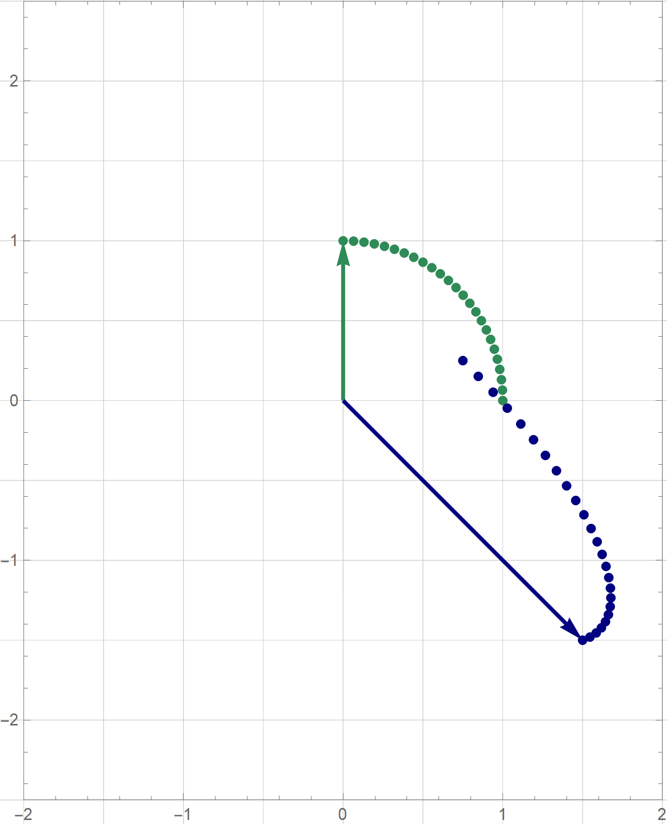
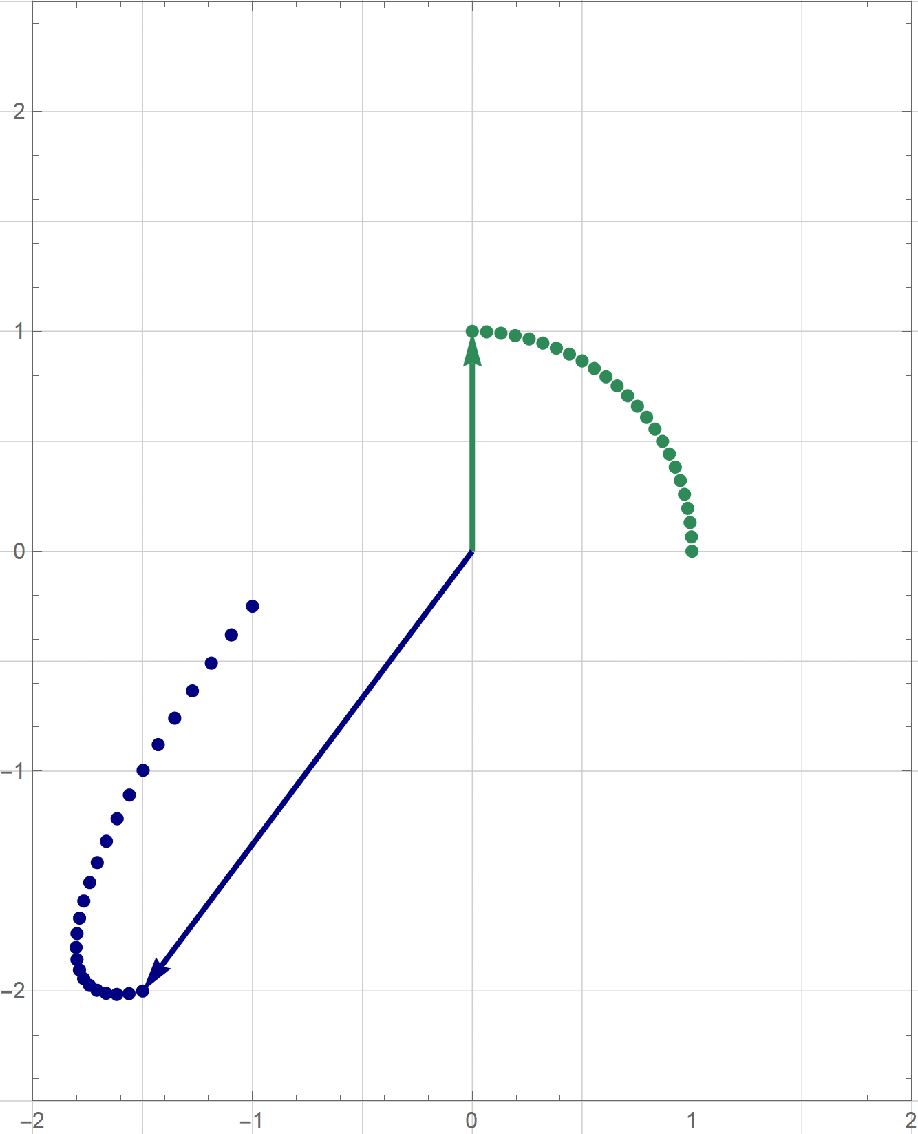
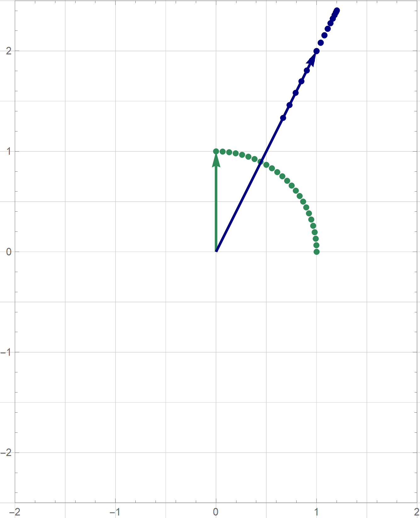
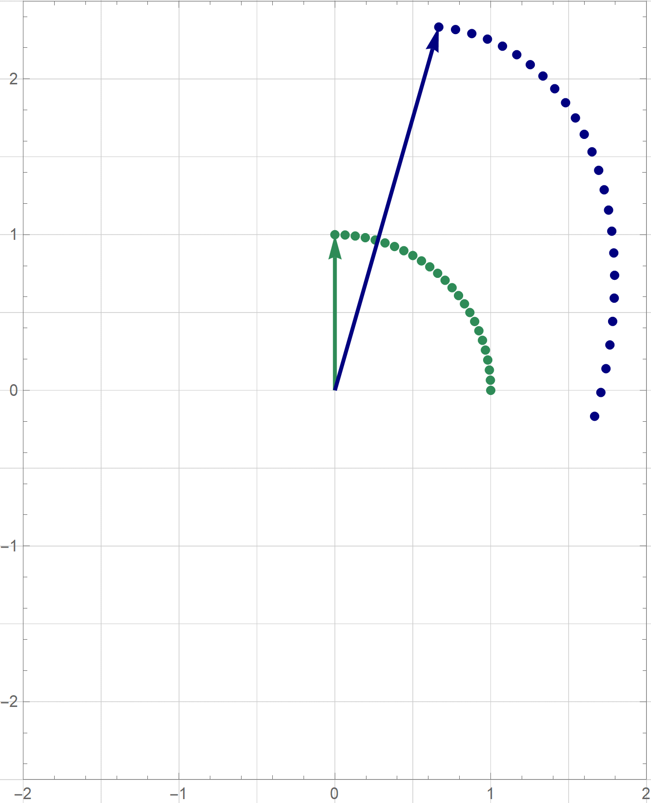
It turns out that the equalities \[ \alpha = a (\cos b) \quad \text{and} \quad \beta = a (\sin b). \] are familiar from Math 224 when we discussed the polar coordinates.
|
|
|
|
For $(\alpha,\beta) \neq (0,0)$, the formulas for $a$ and $b$ are \[ a = \sqrt{\alpha^2 + \beta^2}, \qquad b = \begin{cases} \phantom{-}\arccos\left(\frac{\alpha}{\sqrt{\alpha^2 + \beta^2}}\right) & \text{for} \quad \beta \geq 0, \\[6pt] -\arccos\left(\frac{\alpha}{\sqrt{\alpha^2 + \beta^2}}\right) & \text{for} \quad \beta \lt 0. \end{cases} \] Here $a \gt 0$ and $b \in (-\pi, \pi]$.
We proved two inclusions \[ \operatorname{Span}\bigl\{\sin x, \cos x \bigr\} \subseteq \mathcal{S}_1 \quad \text{and} \quad \mathcal{S}_1 \subseteq \operatorname{Span}\bigl\{\sin x, \cos x \bigr\}. \] Thus, we proved \[ \mathcal{S}_1 = \operatorname{Span}\bigl\{\sin x, \cos x \bigr\}. \] By Theorem 1 in Section 4.1, each span is a subspace. Therefore, $\mathcal{S}_1$ is a subspace.
From the preceding item we have \[ \mathcal{S}_1 = \operatorname{Span}\bigl\{\sin x, \cos x \bigr\}. \] We need to prove that the functions $\sin x, \cos x$ are linearly independent to conclude that $\bigl\{\sin x, \cos x \bigr\}$ is a basis for $\mathcal{S}_1$.
Definition. A nonempty set $\mathcal{V}$ is said to be a vector space over $\mathbb R$ if it satisfies the following 10 axioms.
Explanation of the abbreviations: AE--addition exists, AA--addition is associative, AC--addition is commutative, AZ--addition has zero, AO--addition has opposites, SE-- scaling exists, SA--scaling is associative, SD--scaling distributes over addition of real numbers, SD--scaling distributes over addition of vectors, SO--scaling with one.
Thus, for $u,v \in \mathcal{V}$ the sum of the vectors $u$ and $v$ is denoted by $\mathbf{\mathsf{VectorPlus}}(u,v)$, for $\alpha \in \mathbb{R}$ and $v \in \mathcal{V}$ the scaling of the vector $v$ by $\alpha$ is denoted by $\mathbf{\mathsf{Scale}}(\alpha,v)$, for $\alpha, \beta \in \mathbb{R}$ the sum of the real numbers $\alpha$ and $\beta$ is denoted by $\mathbf{\mathsf{Plus}}(\alpha,\beta)$, and for $\alpha, \beta \in \mathbb{R}$ the product of the real numbers $\alpha$ and $\beta$ is denoted by $\mathbf{\mathsf{Times}}(\alpha,\beta)$.
Just to clarify, in this notation we have $\mathbf{\mathsf{Plus}}(2,3) = 5$ and $\mathbf{\mathsf{Times}}(2,3) = 6$. The distributive law for the real numbers in this notation reads: for all real numbers $\alpha, \beta$ and $\gamma$ we have \[ \mathbf{\mathsf{Times}}\bigl(\alpha, \mathbf{\mathsf{Plus}}(\beta,\gamma) \bigr) = \mathbf{\mathsf{Plus}}\bigl( \mathbf{\mathsf{Times}}(\alpha,\beta) , \mathbf{\mathsf{Times}}(\alpha,\gamma) \bigr) \]
Exercise. Rewrite the axioms SA, SD, SD, and SO using the notation for the algebraic operations introduced above.