-
I updated the notes: The class lecture notes version of May 18, 2024 23:04. I added colored illustrations for the concepts of infimum and supremum in Section 6.3.
-
I updated the notes: The class lecture notes version of May 15, 2024 17:37. I added an illustration for Lemma 6.1.6. This lemma could be nicknamed: split in thirds, emphasize the midpoint.
I also wrote a new proof that \(\mathbb{R}\) is not countable, Theorem 6.1.7. I believe that this proof is the most accessible proof based on First Principle Reasoning.
-
I updated the notes: The class lecture notes version of May 14, 2024 13:08. I wrote Remark 6.1.3 in which I present my reasoning behind the proof that the set \(A\) introduced in the solution for Exercise 6.1.2 does not have a minimum.
I also wrote a new proof that \(\mathbb{R}\) is not countable, Theorem 6.1.6. I believe that this proof is the most accessible proof based on First Principle Reasoning.
-
I updated the notes: The class lecture notes version of May 14, 2024 00:06. I introduced a new subsection Subsection 5.4.2 The Quadruplicity of Sets. In this section I present the case for my quadruplicity of sets.
I also wrote a new proof that \(\mathbb{R}\) is not countable, Theorem 6.1.6. I believe that this proof is the most accessible proof based on First Principle Reasoning.
-
I updated the notes: The class lecture notes version of May 8, 2024 21:27. I introduced a new section Section 5.4 Countable Sets. In this section I give detailed proofs of three theorems Theorem 5.4.2, Theorem 5.4.3, Theorem 5.4.4. Each of these theorems is a powerful tool for proving countability when we cannot construct an explicit bijection between \(\mathbb{N}\) and a set that we want to prove is countable. One of these theorems you are using on the assignment.
I also wrote a new proof that \(\mathbb{R}\) is not countable, Theorem 6.1.6. I believe that this proof is the most accessible proof based on First Principle Reasoning.
-
In today's post, I present a remarkable example of a proof using the Principle of Mathematical Induction. This proof is Example 4.5 in the book:
- Titu Andreescu, Vlad Crsan: Mathematical Induction: A Powerful and Elegant Method of Proof.
-
First recall the exact statement of the Principle of Mathematical Induction.
Principle of Mathematical Induction. By $\mathbb{N}$ we denote the set of positive integers. Let $P(n)$ be a propositional function with $n\in \mathbb{N}$. The following implication holds: \[ P(1) \land \Bigl( \forall \mkern 2mu k \in \mathbb{N} \ \ P(k) \Rightarrow P(k+1) \Bigr) \quad \Rightarrow \quad \forall \mkern 2mu n \in \mathbb{N} \ \ \ P(n) \]
-
Statement of the problem from Andreescu-Crsan book:
Problem 1. Let $\mathbb{R}_{\gt 0}$ denote the set of all positive real numbers. For each $n \in \mathbb{N}$, let $\bigl(\mathbb{R}_{\gt 0}\bigr)^n$ denote the set of all $n$-tuples of positive real numbers. Prove that the following implication holds for all $n\in\mathbb{N}$: \[ \forall \mkern 2mu (a_1,\ldots,a_n) \in \bigl(\mathbb{R}_{\gt 0}\bigr)^n \qquad \prod_{i=1}^n a_i = 1 \quad \Rightarrow \quad n \leq \sum_{i=1}^n a_i . \]
-
Proof.
- Let $n\in\mathbb{N}$. Denote by $P(n)$ the following statement: \[ \forall \mkern 2mu (a_1,\ldots,a_n) \in \bigl(\mathbb{R}_{\gt 0}\bigr)^n \qquad \prod_{i=1}^n a_i = 1 \quad \Rightarrow \quad n \leq \sum_{i=1}^n a_i . \]
- Base case. The statement $P(1)$ reads: \[ \forall \mkern 1mu a_1 \in \mathbb{R}_{\gt 0} \qquad a_1 = 1 \quad \Rightarrow \quad a_1 = 1. \] The preceding implication is clearly true.
-
Inductive step. Let $k\in\mathbb{N}$ be arbitrary. We need to prove \[ P(k) \quad \Rightarrow \quad P(k+1). \] Assume $P(k)$. That is assume \[ \forall \mkern 2mu (b_1,\ldots,b_k) \in \bigl(\mathbb{R}_{\gt 0}\bigr)^k \qquad \prod_{i=1}^k b_i = 1 \quad \Rightarrow \quad k \leq \sum_{i=1}^k b_i. \] The preceding implication is the Inductive hypothesis.
We will prove $P(k+1)$. That is we will prove \[ \forall \mkern 2mu (a_1,\ldots,a_{k+1}) \in \bigl(\mathbb{R}_{\gt 0}\bigr)^{k+1} \qquad \prod_{i=1}^{k+1} a_i = 1 \quad \Rightarrow \quad k+1 \leq \sum_{i=1}^{k+1} a_i. \]
Here is a proof of $P(k+1)$. Let $(a_1,\ldots,a_{k+1}) \in \bigl(\mathbb{R}_{\gt 0}\bigr)^{k+1}$ be arbitrary and assume \[ \prod_{i=1}^{k+1} a_i = 1. \] Since neither product, nor sum depend on the order of the $(k+1)$-tuple, we can also assume that \[ \forall \mkern 1mu i \in \{1,\ldots,k+1\} \quad a_1 \leq a_i \leq a_{k+1}. \] With this order, by Axiom OT, we have \[ a_{k+1} \lt 1 \quad \Rightarrow \quad \forall \mkern 1mu i \in \{1,\ldots,k+1\} \ \ a_i \lt 1 \quad \Rightarrow \quad \prod_{i=1}^{k+1} a_i \lt 1. \] The contrapositive of the implication \[ a_{k+1} \lt 1 \quad \Rightarrow \quad \prod_{i=1}^{k+1} a_i \lt 1 \] is \[ \prod_{i=1}^{k+1} a_i \geq 1 \quad \Rightarrow \quad a_{k+1} \geq 1. \] Since we assume, \[ \prod_{i=1}^{k+1} a_i = 1, \] from the contrapositive, we deduce that $a_{k+1} \geq 1$.
Similarly, the assumed order yields \[ a_{1} \gt 1 \quad \Rightarrow \quad \prod_{i=1}^{k+1} a_i \gt 1. \] The contrapositive of the preceding implication yields that the assumption $\displaystyle \prod_{i=1}^{k+1} a_i = 1$ implies $a_1 \leq 1$.
Notice that \begin{align*} a_1 \leq 1 \ \land \ a_{k+1} \geq 1 &\quad \Rightarrow \quad \bigl(1-a_1\bigr) \bigl(1-a_{k+1}\bigr) \leq 0 \\ &\quad \Rightarrow \quad a_1 a_{k+1} \leq a_1 + a_{k+1} - 1. \end{align*}
Now we use the Inductive hypothesis. To use the Inductive hypothesis we need to define a \(k\)-tuple $(b_1,\ldots,b_k)$. If \(k=1\), we set $(b_1) = (a_1a_{k+1})$. If \(k \gt 1\), let the elements of $(b_1,\ldots,b_k)$ be defined as follows \begin{align*} b_1 & = a_1a_{k+1}, \\ b_i & = a_i \quad \forall \mkern 1mu i \in \{2,\ldots,k\}. \end{align*} Since \[ \prod_{i=1}^k b_i = \prod_{i=1}^{k+1} a_i = 1, \] we can apply the Inductive hypothesis and deduce that \[ k \leq \sum_{i=1}^k b_i. \] Since we proved that \[ b_1 = a_1 a_{k+1} \leq a_1 + a_{k+1} - 1, \] we deduce that \[ k \leq \sum_{i=1}^k b_i = a_1a_{k+1} + \sum_{i=2}^k a_i \leq a_1 + a_{k+1} - 1 + \sum_{i=2}^k a_i. \] Thus, \[ k+1 \leq \sum_{i=1}^{k+1} a_i. \]
-
For completeness, we should specify a necessary and sufficient condition for equality to hold in the inequality described in the above problem.
Problem 2. Let $\mathbb{R}_{\gt 0}$ denote the set of all positive real numbers. For each $n \in \mathbb{N}$, let $\bigl(\mathbb{R}_{\gt 0}\bigr)^n$ denote the set of all $n$-tuples of positive real numbers. Prove that the following implication holds for all $n\in\mathbb{N}$: \[ \forall \mkern 2mu (a_1,\ldots,a_n) \in \mathbb{R}_{\gt 0}^n \qquad \prod_{i=1}^n a_i = 1 \quad \Rightarrow \quad n \leq \sum_{i=1}^n a_i . \] Equality in the last inequality holds if and only if $(a_1,\ldots,a_n) = (1,\ldots,1)$.
-
An application of the above problem provides one of the simplest proofs of the Inequality of Arithmetic and Geometric Means, see the Wikipedia page AM-GM Inequality
Proof.AM-GM Inequality. Let $\mathbb{R}_{\gt 0}$ denote the set of all positive real numbers. For each $n \in \mathbb{N}$, let $\bigl(\mathbb{R}_{\gt 0}\bigr)^n$ denote the set of all $n$-tuples of positive real numbers. Prove that the following implication holds for all $n\in\mathbb{N}$: \[ \forall\mkern 2mu (x_1,\ldots,x_n) \in \bigl(\mathbb{R}_{\gt 0}\bigr)^n \qquad \sqrt[n]{x_1 \cdots x_n} \leq \frac{x_1 + \cdots + x_n}{n}. \] Equality in the last inequality holds if and only if $x_1 = \cdots = x_n$.
- Let $n\in\mathbb{N}$ and $(x_1,\ldots,x_n) \in \mathbb{R}_{\gt 0}^n$ be arbitrary. Set $\alpha = \sqrt[n]{x_1 \cdots x_n}$. Then $\alpha \gt 0$ and $\alpha^n = x_1 \cdots x_n$. Set \[ \forall\mkern 1mu i \in \{1,\ldots,n\} \quad a_i = \frac{x_i}{\alpha}. \] Then, \[ (a_1,\ldots,a_n) \in \bigl(\mathbb{R}_{\gt 0}\bigr)^n \ \ \land \ \ \prod_{i=1}^n a_i = \frac{x_1 \cdots x_n}{\alpha^n} = 1. \] By Problem 1, we deduce that \[ n \leq \sum_{i=1}^n a_i = \frac{1}{\alpha}\bigl( x_1 + \cdots + x_n \bigr). \] Consequently, since $n \gt 0$ and $\alpha \gt 0$, we have \[ \sqrt[n]{x_1 \cdots x_n} = \alpha \leq \frac{1}{n}\bigl( x_1 + \cdots + x_n \bigr). \] This proves the AM-GM inequality.
-
We started with Problem 1 which is a special case of the AM-GM Inequality, then we used Problem 1 to prove the AM-GM Inequality. We could have chosen a different special case of the AM-GM Inequality and formulated it as a problem. The proof is likely similar, though I have not carried it out myself. Therefore, it remains my conjecture for now.
Problem 3. Let $\mathbb{R}_{\gt 0}$ denote the set of all positive real numbers. For each $n \in \mathbb{N}$, let $\bigl(\mathbb{R}_{\gt 0}\bigr)^n$ denote the set of all $n$-tuples of positive real numbers. Prove that the following implication holds for all $n\in\mathbb{N}$: \[ \forall \mkern 2mu (a_1,\ldots,a_n) \in \bigl(\mathbb{R}_{\gt 0}\bigr)^n \qquad \sum_{i=1}^n a_i = n \quad \Rightarrow \quad \prod_{i=1}^n a_i \leq 1. \] Equality in the last inequality holds if and only if $(a_1,\ldots,a_n) = (1,\ldots,1)$.
- I updated the notes: The class lecture notes version of April 26, 2024 14:38. A few small improvements.
- Below I repeat the post of Tuesday with improved animation.
-
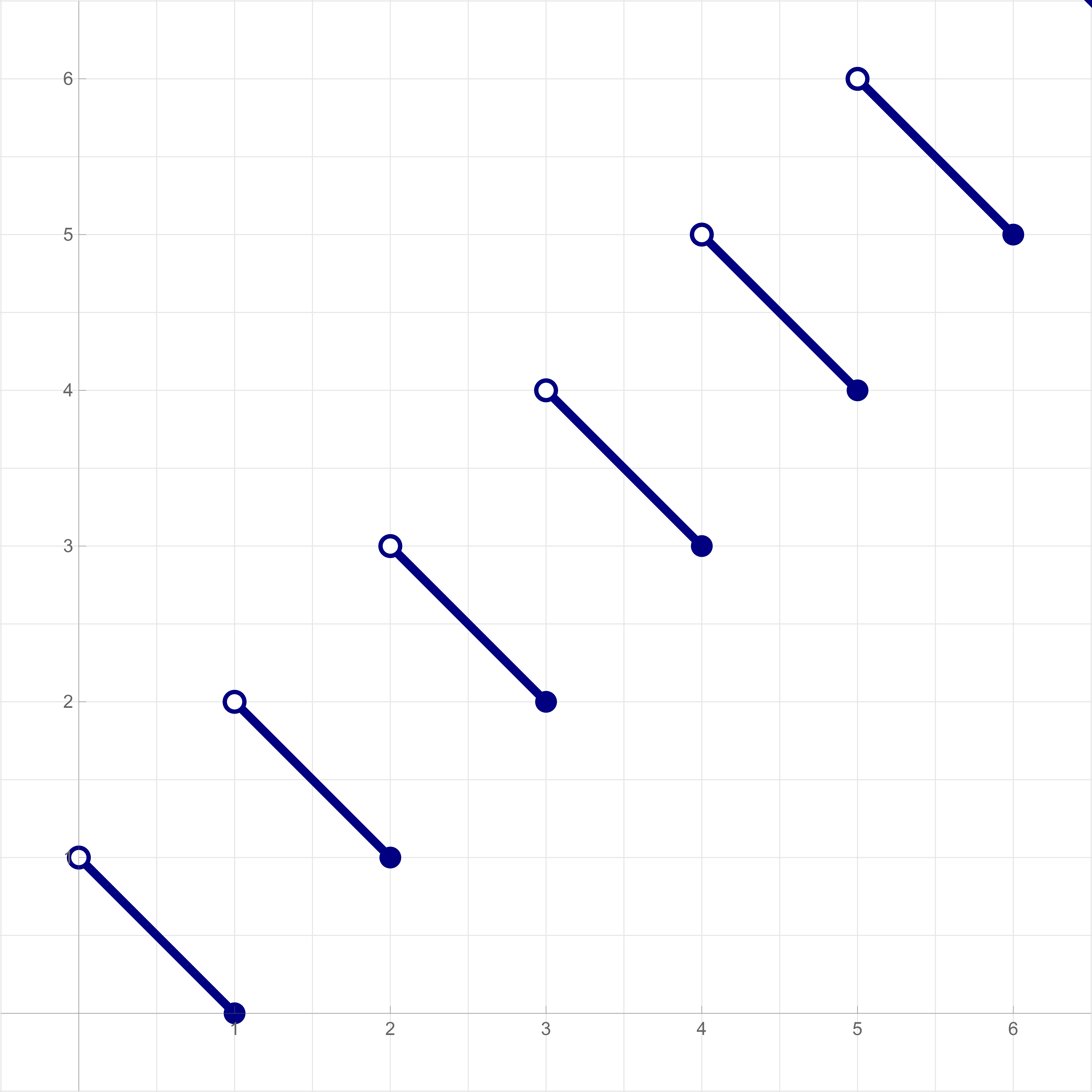
In Subsection 4.3.2 Cardinality of intervals we construct a bijection between any two intervals of real numbers. See the details in the lecture notes. A bijection I find particularly cute is the following one: Its graph is symmetric, it is defined by an intriguing formula, and it is accompanied by an animation I created.
The function with domain \(\mathbb{R}_{\gt 0}\) and range \(\mathbb{R}_{\geq 0}\) given by the formula \[ \forall\mkern+0.5mu x \in \mathbb{R}_{\gt 0} \qquad x \mapsto 2 \lceil x \rceil - 1 - x, \] is a bijection. Its inverse is a function with domain \(\mathbb{R}_{\geq 0}\) and range \(\mathbb{R}_{\gt 0}\) is given by the formula: \[ \forall\mkern+0.5mu x \in \mathbb{R}_{\geq 0} \qquad x \mapsto 2 \lfloor x \rfloor + 1 - x. \] The claim that these two functions are inverses of each other is verified using properties of the floor and ceiling.
\(\forall\mkern+0.5mu x \in \mathbb{R}_{\gt 0} \quad x \mapsto 2 \lceil x \rceil - 1 - x\) 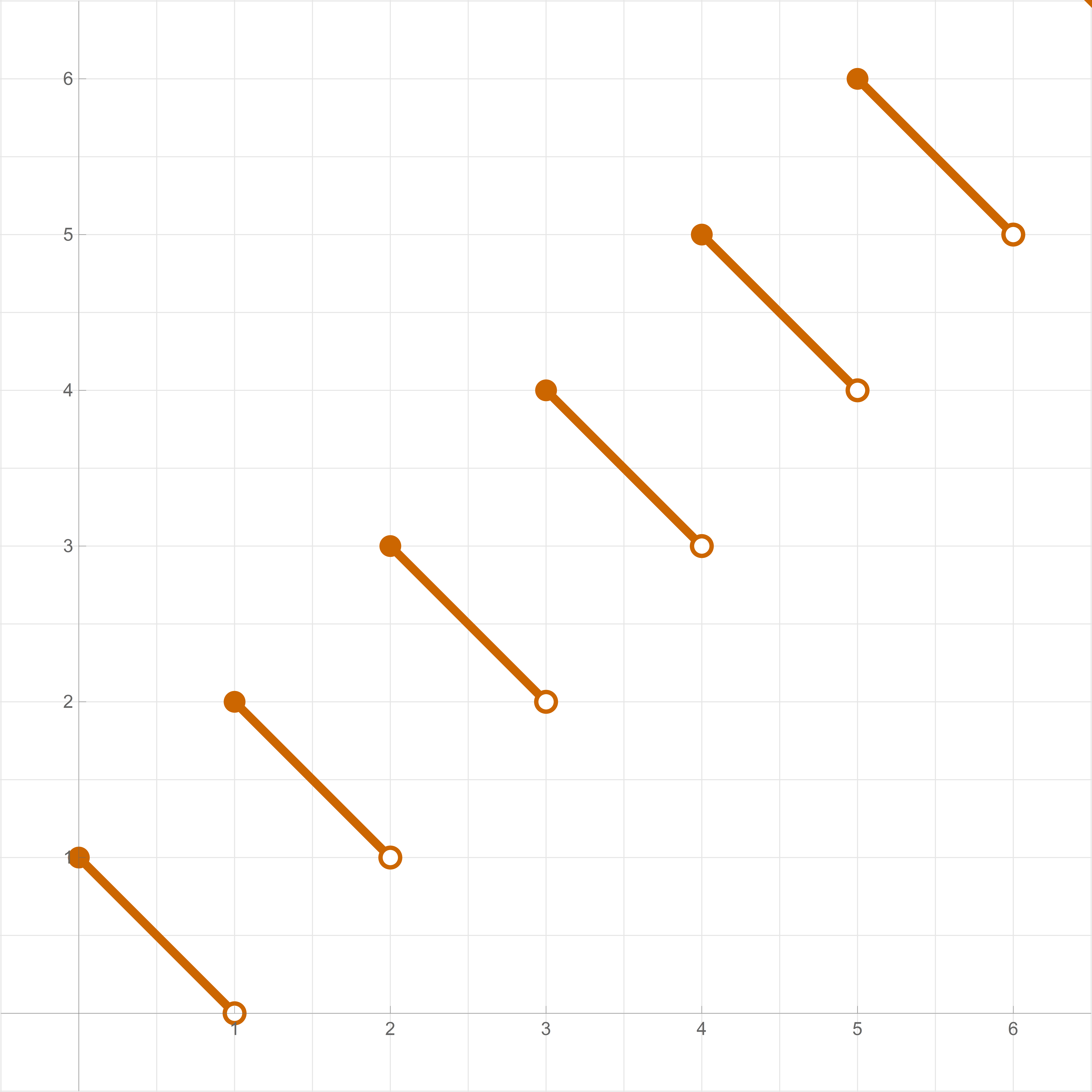
\(\forall\mkern+0.5mu x \in \mathbb{R}_{\geq 0} \quad x \mapsto 2 \lfloor x \rfloor + 1 - x\) The animation below illustrates the action of the blue bijection above on the set of positive real numbers \(\mathbb{R}_{\gt 0}\). The set \(\mathbb{R}_{\gt 0}\) is split into half-open intervals \((n-1,n]\), where \(n \in \mathbb{N}\), the set of positive integers. Then, each of these intervals is flipped about its midpoint. That is the meaning of the blue plot above. The animation starts with the domain, \(\mathbb{R}_{\gt 0}\), the point \(0\) is excluded, signified by the circle placed on the number line at point corresponding to the number \(0\). The animation ends with the range, \(\mathbb{R}_{\geq 0}\), the point \(0\) is included, signified by the disk placed on the number line at the point corresponding to the number \(0\).
Place the cursor over the image to start the animation.

- I updated the notes: The class lecture notes version of April 26, 2024 00:55. I made many small improvements. A major change is that I placed Cantor's Theorem in a Subsection on its own Subsection 3.2.5 Cantor's theorem. Previously, Subsection 3.2.4 Invertible function, inverse was too long, and Cantor's Theorem deserves a subsection in its own right.
-
In Subsection 4.3.2 Cardinality of intervals we construct a bijection between any two intervals of real numbers. See the details in the lecture notes. A bijection I find particularly cute is the following one: Its graph is symmetric, it is defined by an intriguing formula, and it is accompanied by an animation I created.
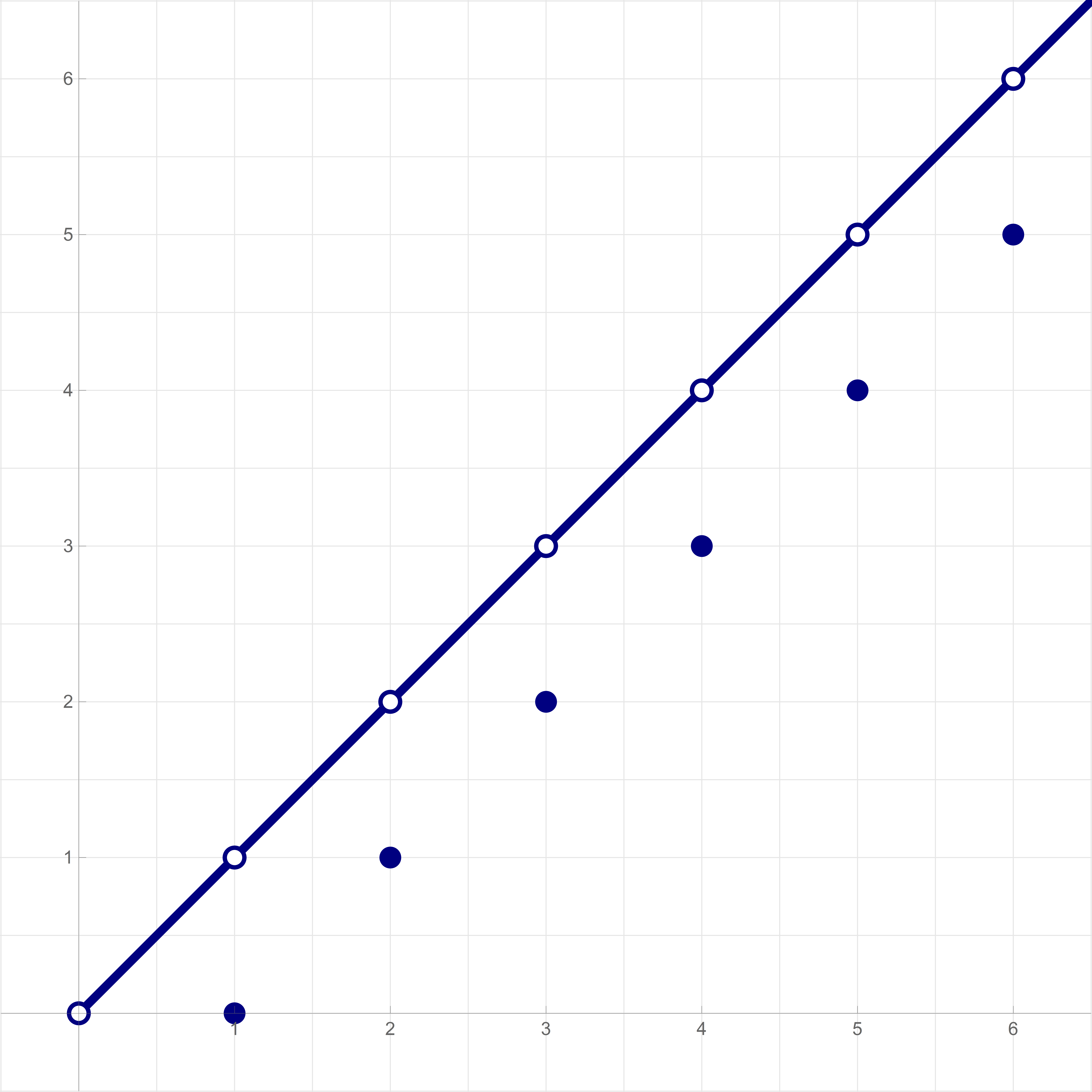
On Tuesday I posted about a beautiful bijection with domain \(\mathbb{R}_{\gt 0}\) and range \(\mathbb{R}_{\geq 0}\). The bijection from Tuesday is mentioned in the lecture notes only in Remark 4.3.12. The main bijection in the lecture notes is the bijection \(\phi: \mathbb{R}_{\gt 0} \to \mathbb{R}_{\geq 0}\) given by the following piecewise formula \[ \forall\mkern+0.5mu x \in \mathbb{R}_{\gt 0} \qquad \phi(x) = \begin{cases} x & \text{if} \mkern+20mu x \in \mathbb{R}_{\gt 0} \setminus \mathbb{N}, \\[3pt] x - 1 & \text{if} \mkern+20mu x\in \mathbb{N}. \end{cases} \] Its inverse \[ \forall\mkern+0.5mu x \in \mathbb{R}_{\geq 0} \qquad \phi^{-1}(x) = \begin{cases} x & \text{if} \mkern+20mu x \in \mathbb{R}_{\gt 0} \setminus \mathbb{N}, \\[3pt] x + 1 & \text{if} \mkern+20mu x\in \mathbb{N}\cup\{0\}, \end{cases} \] is a bijection with domain \(\mathbb{R}_{\geq 0}\) and range \(\mathbb{R}_{\gt 0}\). Below are their graphs.
The bijection \(\phi:\mathbb{R}_{\gt 0}\to \mathbb{R}_{\geq 0}\) 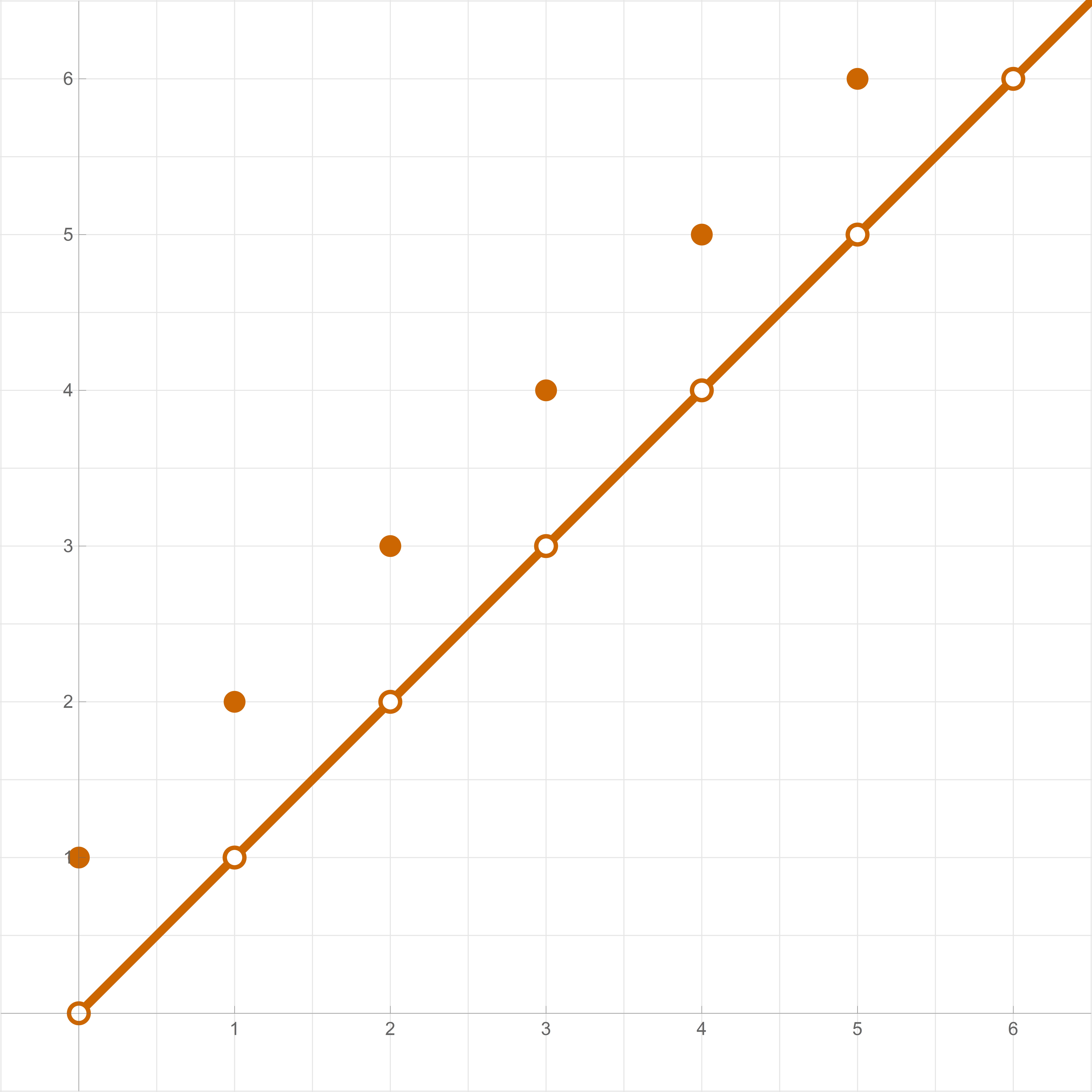
The inverse \(\phi^{-1}:\mathbb{R}_{\geq 0}\to \mathbb{R}_{\gt 0}\) of the bijection \(\phi\) The animation below illustrates the action of the bijection \(\phi\) on the set of positive real numbers \(\mathbb{R}_{\gt 0}\). There is no action on the positive real numbers that are not positive integers. Positive integers are shifted backward. The animation ends with the range, \(\mathbb{R}_{\geq 0}\), the point \(0\) is included, signified by the disk placed on the number line at the point corresponding to the number \(0\).
Place the cursor over the image to start the animation.

- I updated the notes: The class lecture notes version of April 23, 2024 17:02. Many small improvements, many new pictures in Subsection 4.3.2 Cardinality of intervals.
-
In Subsection 4.3.2 Cardinality of intervals we construct a bijection between any two intervals of real numbers. See the details in the lecture notes. A bijection I find particularly cute is the following one: Its graph is symmetric, it is defined by an intriguing formula, and it is accompanied by an animation I created.
The function with domain \(\mathbb{R}_{\gt 0}\) and range \(\mathbb{R}_{\geq 0}\) given by the formula \[ \forall\mkern+0.5mu x \in \mathbb{R}_{\gt 0} \qquad x \mapsto 2 \lceil x \rceil - 1 - x, \] is a bijection. Its inverse is a function with domain \(\mathbb{R}_{\geq 0}\) and range \(\mathbb{R}_{\gt 0}\) is given by the formula: \[ \forall\mkern+0.5mu x \in \mathbb{R}_{\geq 0} \qquad x \mapsto 2 \lfloor x \rfloor + 1 - x. \] The claim that these two functions are inverses of each other is verified using properties of the floor and ceiling.

\(\forall\mkern+0.5mu x \in \mathbb{R}_{\gt 0} \quad x \mapsto 2 \lceil x \rceil - 1 - x\) 
\(\forall\mkern+0.5mu x \in \mathbb{R}_{\geq 0} \quad x \mapsto 2 \lfloor x \rfloor + 1 - x\) The animation below illustrates the action of the blue bijection above on the set of positive real numbers \(\mathbb{R}_{\gt 0}\). The set \(\mathbb{R}_{\gt 0}\) is split into half-open intervals \((n-1,n]\), where \(n \in \mathbb{N}\), the set of positive integers. Then, each of these intervals is flipped about its midpoint. That is the meaning of the blue plot above. The animation starts with the domain, \(\mathbb{R}_{\gt 0}\), the point \(0\) is excluded, signified by the circle placed on the number line at point corresponding to the number \(0\). The animation ends with the range, \(\mathbb{R}_{\geq 0}\), the point \(0\) is included, signified by the disk placed on the number line at the point corresponding to the number \(0\).
Place the cursor over the image to start the animation.

- I updated the notes: The class lecture notes version of April 21, 2024 22:52. I finished rewriting Chapter Four on The set \(\mathbb{R}\) of real numbers. I wrote new Section 4.2 Four functions to start with and Section 4.3 Intervals. In particular, the long Subsection 4.3.2 Cardinality of intervals is completely new.
- I updated the notes: The class lecture notes version of April 19, 2024 00:48. I rewrote Section 4.1 Axioms of the set \(\mathbb{R}\) of real numbers. This is the first section of Chapter Four on The set \(\mathbb{R}\) of real numbers.
-
In this class, and in all my classes, I emphasize reasoning from First Principles. Solving mathematical problems typically involves utilizing knowledge of related mathematical results. Often, the key to a solution is hidden within these results. I believe that for a solution to be complete, the dependency on related results should be made clear. Effort should be directed towards minimizing the use of related results and replacing them with direct reasoning from First Principles. Discovering First Principles in real-life problems can be challenging; however, in mathematics, they are more accessible and are usually based on Axioms or Fundamental Theorems.
Knowledge built on First Principles is both more robust and more adaptable to new situations. Working from First Principles helps prevent unnecessary complexities in solutions and acts as a safeguard against circular reasoning.
-
As an illustration of First Principle reasoning, I will prove here that the square of a rational number cannot equal \(2\). You can read the proof given by Student5 in Discussions on Canvas which proves this same theorem using two theorems from number theory. Student7 proved a more general theorem: that for all positive integers \(n\) we have that \(\sqrt{n}\) is rational if and only if \(n\) is a square of an integer. This student used the Fundamental Theorem of Arithmetic in the proof. The proof given by Student5 and my proof below, can be adopted to prove that \(\sqrt{p}\) is irrational for a prime \(p\). I don't think that theorem proven by Student7 can be done without the Fundamental Theorem of Arithmetic.
Theorem. Irrationality of \(\sqrt{2}\). For every \(r \in \mathbb{Q}\) we have \(r^2 \neq 2\).
-
We start with the Background Knowledge.
BK1. We assume that the reader is familiar with the algebra in the set of integers \(\mathbb{Z}\). Note that by \(\mathbb{N}\) we denote the set of positive integers and both \(\mathbb{Z}\) and \(\mathbb{N}\) are subsets of the real numbers \(\mathbb{R}\).
BK2. We consider the set of even integers \(\mathbb{E}\) defined as \[ \mathbb{E} = \bigl\{ n \in \mathbb{Z} : \exists \mkern+1.5mu k \in \mathbb{Z} \ \ n = 2 k \bigr\}, \] and the set of odd integers \(\mathbb{O}\) defined as \[ \mathbb{O} = \bigl\{ n \in \mathbb{Z} : \exists \mkern+1.5mu k \in \mathbb{Z} \ \ n = 2 k + 1 \bigr\}. \] Two facts about odd and even integers are \[ \mathbb{Z} = \mathbb{E} \cup \mathbb{O} \quad \text{and} \quad \mathbb{E} \cap \mathbb{O} = \emptyset. \] For all \(n \in \mathbb{Z}\) we have \(n \in \mathbb{E}\) if and only if \(n^2 \in \mathbb{E}\).
BK3. Definition of rational numbers \(\mathbb{Q}\): \[ \mathbb{Q} = \left\{ x \in \mathbb{R} : \exists\mkern+1.5mu m \in \mathbb{Z} \ \land \ \exists\mkern+1.5mu n \in \mathbb{N} \quad x = \frac{m}{n} \right\} \]
BK4. Well Ordering Axiom (WOA). The First Principle in this context is the Well Ordering Axiom (WOA): Every nonempty subset of \(\mathbb{N}\) has a minimum. Or, in the notation of formal logic \[ S \subset \mathbb{N} \land S \neq \emptyset \quad \Rightarrow \quad \exists\mkern+1.5mu m \in S \ \ \forall\mkern+0.5mu x \in S \ \ m \leq x. \]
BK5. Proof by contradiction. Let \(p\) be a proposition that we need to prove. The logic of a proof by contradiction goes as follows. We assume that the negation of \(\lnot p\) is true. Then we pursue logically correct reasoning and prove that the following implication is true: \[ (\lnot p) \Rightarrow \mathsf{F}. \] In any specific example, \(\mathsf{F}\) is a specific False statement. For example, in the proof that \(\sqrt{2}\) is not rational, we will prove the negation of WOA. Thus, we will prove \[ (\lnot p) \Rightarrow \lnot (\operatorname{WOA}). \] As, the preceding implication is true, its contrapositive is true as well. Thus, we have proved \[ \operatorname{WOA} \Rightarrow p. \] Thus, \(p\) is proved.
In summary, by proving \((\lnot p) \Rightarrow \mathsf{F}\), we have proved its contrapositive \(\mathsf{T} \Rightarrow p\), which means that \(p\) is true.
-
Step 1. We will prove the claim by a proof by contradiction, see BK5. Assume that the negation of the statement in the theorem is true. That is assume: \[ \exists\mkern+1.5mu r \in \mathbb{Q} \quad r^2 = 2. \] By BK3 there exist \(m \in \mathbb{Z}\) and \(n \in \mathbb{N}\) such that \(r = m/n\). Therefore \[ \require{bbox} \bbox[5px, #88FF88, border: 1pt solid green]{ \exists\mkern+1.5mu m \in \mathbb{Z} \ \ \exists\mkern+1.5mu n \in \mathbb{N} \qquad m^2 = 2 n^2.} \]
Step 2. Let us now consider the set \[ S = \left\{ q \in \mathbb{N} : \exists\mkern+1.5mu p \in \mathbb{Z} \quad p^2 = 2 q^2 \right\} \] By the green box at the end of Step 1, we deduce that \(n \in S\). Therefore, \(\bbox[5px, #88FF88, border: 1pt solid green]{S\neq \emptyset}\).
Step 3. Now we will prove that \(S\) does not have a minimum. That is we will prove \[ \forall\mkern+0.5mu q \in S \ \ \exists\mkern+1.5mu l \in S \qquad l \lt q. \] Let \(q \in S\) be arbitrary. By the definition of \(S\), there exists \(p \in \mathbb{Z}\) such that \(p^2 = 2 q^2\). The last equality implies that $p^2 \in \mathbb{E}$. By BK2 we have that \(p \in \mathbb{E}\). Since \(p \in \mathbb{E}\), there exists \(k \in \mathbb{Z}\) such that \(p = 2k\). Since \(p^2 = 2 q^2\), we also have \(4 k^2 = 2 q^2\). Consequently, \(q^2 = 2 k^2\). Thus, \(q^2\) and, by BK2, also \(q\) is even. Hence, there exists \(l \in \mathbb{N}\) such that \(q = 2 l\). Since \(q, l \in \mathbb{N}\), we have \(l \lt q\). Since \(q^2 = 2 k^2\), we also have \(4 l^2 = 2 k^2\), that is \( k^2 = 2 l^2\). Since \(l \in\mathbb{N}\), we have \(l \in S\). In conclusion, we proved that \[ \require{bbox} \bbox[5px, #88FF88, border: 1pt solid green]{ \forall\mkern+0.5mu q \in S \ \ \exists\mkern+1.5mu l \in S \quad l \lt q.} \]
Step 4. In Step 2 we proved that \(S\neq \emptyset\). In Step 3 we proved that \(S\) does not have a minimum. Thus, we have proved the negation of the Well Ordering Axiom. That is, we proved, \[ \require{bbox} \bbox[5px, #88FF88, border: 1pt solid green]{ \exists\mkern+1.5mu r \in \mathbb{Q} \quad r^2 = 2 \quad \Rightarrow \quad \lnot (\operatorname{WOA}). } \] Thus, the contrapositive of the preceding green box is also true: \[ \require{bbox} \bbox[5px, #88FF88, border: 1pt solid green]{ \operatorname{WOA} \quad \Rightarrow \quad \forall\mkern+1.5mu r \in \mathbb{Q} \quad r^2 \neq 2 . } \] This completes the proof.
- I updated the notes: The class lecture notes version of April 16, 2024 21:28. I finished short section Section 3.3 Cardinality of sets. That completes Chapter Three on Sets and Functions.
- On Thursday we will discuss Cantor's theorem, Theorem 3.2.21, which we started today, and talk about cardinality of infinite sets. That would complete Chapter Three on Sets and Functions. On Friday we move on to Chapter Four on The set \(\mathbb{R}\) of Real Numbers.
-
Definition. Let $A$ and $B$ be two nonempty sets. The set of all functions $f: A \to B$ with domain $A$ and codomain $B$ is denoted by $B^A$.
The reason for this notation is that if the set $A$ has $m$ elements and the set $B$ has $n$ elements, then the set $B^A$ has $n^m$ elements. For example, if $A=\{\blacktriangle,\blacksquare\}$ and $B=\{1,2,3\}$ then we can list all the functions from $A$ to $B$ in a table:
$f_1$ $f_2$ $f_3$ $f_4$ $f_5$ $f_6$ $f_7$ $f_8$ $f_9$ $\blacktriangle$ $1$ $1$ $1$ $2$ $2$ $2$ $3$ $3$ $3$ $\blacksquare$ $1$ $2$ $3$ $1$ $2$ $3$ $1$ $2$ $3$ Or, it might be more interesting to make \(B=\{\color{#EE0000}{\mathbf{R}}, \color{#00CC00}{\mathbf{G}}, \color{#0000EE}{\mathbf{B}}\}\), the set of the primary colors, RED, GREEN and BLUE. Then the list of functions is as follows:
Or, representing the value of a function on a shape by coloring that shape with the function color value:$f_1$ $f_2$ $f_3$ $f_4$ $f_5$ $f_6$ $f_7$ $f_8$ $f_9$ $\blacktriangle$ $\color{#EE0000}{\mathbf{R}}$ $\color{#EE0000}{\mathbf{R}}$ $\color{#EE0000}{\mathbf{R}}$ $\color{#00CC00}{\mathbf{G}}$ $\color{#00CC00}{\mathbf{G}}$ $\color{#00CC00}{\mathbf{G}}$ $\color{#0000EE}{\mathbf{B}}$ $\color{#0000EE}{\mathbf{B}}$ $\color{#0000EE}{\mathbf{B}}$ $\blacksquare$ $\color{#EE0000}{\mathbf{R}}$ $\color{#00CC00}{\mathbf{G}}$ $\color{#0000EE}{\mathbf{B}}$ $\color{#EE0000}{\mathbf{R}}$ $\color{#00CC00}{\mathbf{G}}$ $\color{#0000EE}{\mathbf{B}}$ $\color{#EE0000}{\mathbf{R}}$ $\color{#00CC00}{\mathbf{G}}$ $\color{#0000EE}{\mathbf{B}}$ $f_1$ $f_2$ $f_3$ $f_4$ $f_5$ $f_6$ $f_7$ $f_8$ $f_9$ $\blacktriangle$ $\color{#EE0000}{\blacktriangle}$ $\color{#EE0000}{\blacktriangle}$ $\color{#EE0000}{\blacktriangle}$ $\color{#00CC00}{\blacktriangle}$ $\color{#00CC00}{\blacktriangle}$ $\color{#00CC00}{\blacktriangle}$ $\color{#0000EE}{\blacktriangle}$ $\color{#0000EE}{\blacktriangle}$ $\color{#0000EE}{\blacktriangle}$ $\blacksquare$ $\color{#EE0000}{\blacksquare}$ $\color{#00CC00}{\blacksquare}$ $\color{#0000EE}{\blacksquare}$ $\color{#EE0000}{\blacksquare}$ $\color{#00CC00}{\blacksquare}$ $\color{#0000EE}{\blacksquare}$ $\color{#EE0000}{\blacksquare}$ $\color{#00CC00}{\blacksquare}$ $\color{#0000EE}{\blacksquare}$ - Why am I playing with colors here? To some extend, I believe that all functions are colorings. Sometimes you have to have a lot of colors. And, you have to respect the rule not to color a single object in the domain by two colors. That is, stay `unival'. And, you have to respect the rule to color each and every object in the domain. That is, be `total'.
-
In the above example, I have $2$ shapes and $3$ colors. So, I can color the first shape in three colors and the second shape in three colors. So, I can color the shapes in $3 \times 3$ ways. If I had $m$ distinct shapes and $n$ distinct colors, then I could color the shapes in $n \times n \times \cdots \times n$ ways; the total of $n^m$ ways. This reasoning is known as the rule of product counting principle. This counting is the reason why the set of all functions $f:A\to B$ with domain $A$ and codomain $B$ is denoted as \[ B^{\Large A} \qquad (n \ \text{colors})^{m \ \text{shapes}} \]
-
In class I proved
Proposition 3.2.17. For an arbitrary nonempty set $S$ there exist a bijection between the power set of $S$ and the set $\{0,1\}^S$.
The table below illustrates the proof. Consider $S=\{\blacktriangle,\diamond,\bullet,\star\}$. The table below indicates what the bijection should be. The top part of the table contains sixteen functions in $\{0,1\}^S$; the bottom part contains the subsets of $A$ that are related to the functions above them.
$f_1$ $f_2$ $f_3$ $f_4$ $f_5$ $f_6$ $f_7$ $f_8$ $f_9$ $f_{10}$ $f_{11}$ $f_{12}$ $f_{13}$ $f_{14}$ $f_{15}$ $f_{16}$ $\blacktriangle$ $0$ $0$ $0$ $0$ $0$ $0$ $0$ $0$ $1$ $1$ $1$ $1$ $1$ $1$ $1$ $1$ $\diamond$ $0$ $0$ $0$ $0$ $1$ $1$ $1$ $1$ $0$ $0$ $0$ $0$ $1$ $1$ $1$ $1$ $\bullet$ $0$ $0$ $1$ $1$ $0$ $0$ $1$ $1$ $0$ $0$ $1$ $1$ $0$ $0$ $1$ $1$ $\star$ $0$ $1$ $0$ $1$ $0$ $1$ $0$ $1$ $0$ $1$ $0$ $1$ $0$ $1$ $0$ $1$ s u b s e t$\emptyset$ $\{\star\}$ $\{\bullet\}$ $\left\{\begin{array}{c}\!\!\bullet\!\!\\\!\!\star\!\! \end{array}\right\}$ $\{\diamond\}$ $\left\{\begin{array}{c}\!\!\diamond\!\!\\\!\!\star\!\!\end{array}\right\}$ $\left\{\begin{array}{c}\!\!\diamond\!\!\\\!\!\bullet\!\!\end{array}\right\}$ $\left\{\begin{array}{c}\!\!\diamond\!\!\\\!\!\bullet\!\!\\\!\!\star\!\! \end{array}\right\}$ $\{\blacktriangle\}$ $\left\{\begin{array}{c}\!\!\blacktriangle\!\!\\\!\!\star\!\!\end{array}\right\}$ $\left\{\begin{array}{c}\!\!\blacktriangle\!\!\\\!\!\bullet\!\! \end{array}\right\}$ $\left\{\begin{array}{c}\!\!\blacktriangle\!\!\\\!\!\bullet\!\!\\\!\!\star\!\! \end{array}\right\}$ $\left\{\begin{array}{c}\!\!\blacktriangle\!\!\\\!\!\diamond\!\! \end{array}\right\}$ $\left\{\begin{array}{c}\!\!\blacktriangle\!\!\\\!\!\diamond\!\!\\\!\!\star\!\! \end{array}\right\}$ $\left\{\begin{array}{c}\!\!\blacktriangle\!\!\\\!\!\diamond\!\!\\\!\!\bullet\!\! \end{array}\right\}$ $\left\{\begin{array}{c}\!\!\blacktriangle\!\!\\\!\!\diamond\!\!\\\!\!\bullet\!\!\\\!\!\star\!\! \end{array}\right\}$ The function \[ \Phi: \mathcal{P}(S) \to \{0,1\}^S \] defined in the proof of Proposition 3.2.17 is given in the columns of the above table. For example, in the above table, if $A = \{\blacktriangle,\bullet,\star\}$, then $\Phi(A) = f_{12}$, that is the function \[ f_{12}(\blacktriangle)=1, \quad f_{12}(\diamond)=0, \quad f_{12}(\bullet)=1, \quad f_{12}(\star)=1. \]
-
Recall Cantor's Theorem, that is Theorem 3.2.21 in the lecture notes:
Cantor's Theorem. Let $S$ be a nonempty set. Then there is no surjection with domain $S$ and codomain $\mathcal{P}(S)$.
In the proof of this theorem we prove \[ \forall\mkern+1.2mu \Theta: S \to \mathcal{P}(S) \quad \exists\mkern+1.5mu G \subseteq S \quad \forall\mkern+1.2mu x \in S \quad \Theta(x) \neq G. \] To prove the preceding displayed statement, let $\Theta: S \to \mathcal{P}(S)$ be an arbitrary function with domain \(S\) and codomain \(\mathcal{P}(S)\). To prove that $\Theta$ is not a surjection, we need to discover a subset $G$ of $S$ such that \[ \forall\mkern+1.2mu x \in S \quad \Theta(x) \neq G. \] The definition of such subset $G$ is truly ingenious, due to Georg Cantor: \[ G = \bigl\{ s \in S : s \not\in \Theta(s) \bigr\}. \]
-
I want to illustrate the universality of the definition of \(G\) on the example considered in the preceding item. Let \[ S=\{\blacktriangle,\diamond,\bullet,\star\}. \]
-
Next, I need to select a function \(\Theta: S \to \mathcal{P}(S)\). I randomly choose:
\[
\Theta(\blacktriangle) = \{\blacktriangle,\star\}, \quad
\Theta(\diamond) =\{\bullet,\star\} , \quad
\Theta(\bullet) = \{\blacktriangle,\bullet\}, \quad
\Theta(\star) = \{\bullet\}.
\]
Now, I construct the set \(G\), by asking:
- Is \(\blacktriangle \in G\)? That is, is \(\blacktriangle \in \Theta(\blacktriangle)\)? Yes. Thus, \(\blacktriangle \not\in G\)?
- Is \(\diamond \in G\)? That is, is \(\diamond \in \Theta(\diamond)\)? No. Thus, \(\diamond \in G\)?
- Is \(\bullet \in G\)? That is, is \(\bullet \in \Theta(\bullet)\)? Yes. Thus, \(\bullet \not\in G\)?
- Is \(\star \in G\)? That is, is \(\star \in \Theta(\star)\)? No. Thus, \(\star \in G\)?
-
Now I select a different function \(\Theta: S \to \mathcal{P}(S)\). I randomly choose:
\[
\Theta(\blacktriangle) = \{\blacktriangle,\diamond,\star\}, \quad
\Theta(\diamond) =\{\blacktriangle,\diamond,\bullet\} , \quad
\Theta(\bullet) = \{\star\}, \quad
\Theta(\star) = \{\blacktriangle, \star \}.
\]
Now, I construct the set \(G\), by asking:
- Is \(\blacktriangle \in G\)? That is, is \(\blacktriangle \in \Theta(\blacktriangle)\)? Yes. Thus, \(\blacktriangle \not\in G\)?
- Is \(\diamond \in G\)? That is, is \(\diamond \in \Theta(\diamond)\)? Yes. Thus, \(\diamond \not\in G\)?
- Is \(\bullet \in G\)? That is, is \(\bullet \in \Theta(\bullet)\)? No. Thus, \(\bullet \in G\)?
- Is \(\star \in G\)? That is, is \(\star \in \Theta(\star)\)? Yes. Thus, \(\star \not\in G\)?
- Two specific examples show the universality of the definition of \(G\). And, in the proof of Theorem 3.2.21 in the lecture notes, we demonstrated the for arbitrary nonempty set \(S\) and arbitrary \(\Theta: S \to \mathcal{P}(S)\), with \(G \subset S\) defined as \[ G = \bigl\{ s \in S : s \not\in \Theta(s) \bigr\}, \] we have \[ \forall\mkern+1.2mu x \in S \quad \Theta(x) \neq G. \]
- For a finite set \(S\) with \(n\) elements, the set \(\mathcal{P}(S)\) has \(2^n\) elements. Since for all \(n \in \mathbb{N}\) we have \(n \lt 2^n\), we could pursue a counting type proof that no surjection exists with domain \(S\) and codomain \(\mathcal{P}(S)\). But, for infinite sets, it is not clear that no such surjection exists.
- Using the concept of cardinality of sets, we proved that for every nonempty set \(S\) the cardinality of \(S\) is strictly smaller that the cardinality of \(\mathcal{P}(S)\). See Theorem 3.3.5 in the lecture notes, which is another version of Cantor's Theorem.
-
- I updated the notes: The class lecture notes version of April 14, 2024 12:13. I wrote Subsection 3.2.4 Invertible function, inverse, a long, interesting subsection. It need to update Section 3.3 Cardinality of sets, a very short section. That will complete Chapter Three on Sets and Functions.
-
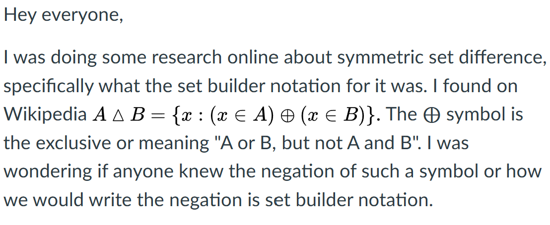
Warren asked an excellent question in Discussions on Canvas:
-
First we recall the definition of the logical equivalence. Let \(p\) and \(q\) be propositions. The equivalence of \(p\) and \(q\), denoted by \(p\Leftrightarrow q\), is defined as the conjunction of the implication \(p\Rightarrow q\) and its converse \(q\Rightarrow p\). That is
\[
(p\Rightarrow q) \land (q\Rightarrow p).
\]
The expression \(p\Leftrightarrow q\) is read "\(p\) if and only if \(q\)." Here is its complete truth table of the definition:
$p$ $q$ $p \Rightarrow q$ $q \Rightarrow p$ $(p\Rightarrow q) \land (q\Rightarrow p)$ $p \Leftrightarrow q$ F F T T T T F T T F F F T F F T F F T T T T T T -
A popular notation for the exclusive disjunction is \(\oplus\), the \(\LaTeX\) code \oplus. Below is the truth table of the exclusive disjunction, its negation, and of the logical equivalence. From this truth table, we can see that the negation of the exclusive disjunction is identical to the logical equivalence. That is \(\lnot(p \oplus q)\) is identical to \(p \Leftrightarrow q\).
$p$ $q$ $p \oplus q$ $\lnot(p \oplus q)$ $p \Leftrightarrow q$ F F F T T F T T F F T F T F F T T F T T - This is a short Intermezzo. The following equivalence is quite clear: \[ (p \Leftrightarrow q) \quad \Leftrightarrow \quad \bigl( (\lnot p) \Leftrightarrow (\lnot q) \bigr) \] Therefore, the negations are also equivalent \[ \lnot (p \Leftrightarrow q) \quad \Leftrightarrow \quad \lnot \bigl( (\lnot p) \Leftrightarrow (\lnot q) \bigr). \] That is \[ p \oplus q \quad \Leftrightarrow \quad (\lnot p) \oplus (\lnot q) \]
- As Warren points out in the question, the exclusive disjunction is a convenient tool to write the symmetric difference in set-builder notation. \[ A \Delta B = \Bigl\{ x \in U : \bigl( x \in A \bigr) \oplus \bigl( x \in B \bigr) \Bigr\}. \]
- Now back to Warren's question: How to express the complement of the symmetric difference in set-builder notation?
- But first some notation. We mentioned at the beginning of our discussion of sets that the core of the meaning of the concept of a set \(S\) is that the expression \(x\in S\) is a proposition, that is, it is either True or False. We introduced the following equivalent expressions \[ \lnot (x \in S) \qquad x\not\in S \qquad x \in S^c. \] In this context one needs to review set-builder notation. Let \(P(x)\) be a propositional function defined on the universe of discourse \(U\). Then, the expression \[ S = \bigl\{ x \in U : P(x) \bigr\} \] means \[ x \in S \quad \Leftrightarrow \quad P(x). \] Therefore \[ S^c = \bigl\{ x \in U : x \not\in S \bigr\} = \bigl\{ x \in U : \lnot P(x) \bigr\}. \]
- Using the equivalent expressions from the preceding item, we have \begin{align*} (A \Delta B)^c & = \Bigl\{ x \in U : \lnot \bigl( \bigl( x \in A \bigr) \oplus \bigl( x \in B \bigr) \bigr) \Bigr\} \\ & = \Bigl\{ x \in U : \bigl( x \in A \bigr) \Leftrightarrow\bigl( x \in B \bigr) \Bigr\} \end{align*}
- Since \[ p \Leftrightarrow q \qquad \Leftrightarrow \qquad (p \land q) \lor (\lnot p \land \lnot q), \] the last set-builder expression for the complement of \(A \Delta B\), shows that the following set equality holds \begin{equation*} (A \Delta B)^c = (A\cap B) \cup \bigl(A^c\cap B^c\bigr) = \bigl( (A^c) \Delta (B^c) \bigr)^c. \end{equation*} Therefore, \begin{equation*} A \Delta B = (A^c) \Delta (B^c) . \end{equation*} I was not aware that this simple symmetry holds for the symmetric set difference. Although, when I think about it, I could have seen it from the definition, written a little differently from what I did. First recall \begin{align*} A \setminus B & = \bigl\{ x \in U : x \in A \land x \not\in B \bigr\} = A\cap B^c, \\ B \setminus A & = \bigl\{ x \in U : x \not\in A \land x \in B \bigr\} = B\cap A^c. \end{align*} Then \begin{align*} A\Delta B & = ( A \cap B^c ) \cup ( B \cap A^c ) \\ & = (A^c \cap B) \cup (B^c \cap A) \\ & = \bigl( A^c \cap (B^c)^c \bigr) \cup \bigl( B^c \cap (A^c)^c ) \\ & = (A^c) \Delta (B^c). \end{align*}
-
First we recall the definition of the logical equivalence. Let \(p\) and \(q\) be propositions. The equivalence of \(p\) and \(q\), denoted by \(p\Leftrightarrow q\), is defined as the conjunction of the implication \(p\Rightarrow q\) and its converse \(q\Rightarrow p\). That is
\[
(p\Rightarrow q) \land (q\Rightarrow p).
\]
The expression \(p\Leftrightarrow q\) is read "\(p\) if and only if \(q\)." Here is its complete truth table of the definition:
-
I updated the notes today. I corrected some typos and improved formatting. I did not change the labeling of the four conditions in Subsection 3.2.3. Surjection, injection, bijection (via flip). In class, I suggested that the better labels would be as follows:
- Instead of the label Fun 1, in class I suggested that we could use Tot as an abbreviation for the name total which I gave for the fact that a function is required to be defined on the totality of its domain.
- Instead of label Fun 2, in class I suggested that we could use Uni as an abbreviation for the name unival that I gave for fact that a function does a unique assignment of the outputs to the inputs.
- Instead of Inv 1, in class I suggested that we could use Sur, as an abbreviation for the fact that this condition defines a surjection.
- Instead of Inv 2, in class I suggested that we could use Inj as an abbreviation for the fact that this condition defines an injection.
- I still need to write an answer to Warren's excellent question in Discussions on Canvas. Thank you, Warren!
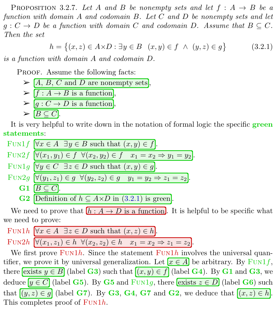
- I updated proof of Proposition 3.2.7, now it is complete, and completely in color. I also proved Proposition 3.2.8, I used less colors and transitioned to a more traditional proof. I wrote Subsection 3.2.3. Surjection, injection, bijection (via flip). I think that I did some interesting writing in this subsection. Please post in Discussions on Canvas if anything is not clear, errors, or suggestions for improvement.
-
I wrote the first part of the proof that we did today. Below is a snippet from the relevant page from the notes. The second part will follow tonight. You can try to prove the second part yourself. I did a lot of labeling. I hope that I am completely detailed in this proof. It is not common to be this detailed. But, we choose to which level of detail we want our proofs presented. Whenever you want more detail, please ask.
- Until I update Section 3.2 Functions of Chapter Three on Sets and Functions, read my webpage Functions.
- I updated the notes: The class lecture notes version of April 8, 2024 16:44. I revised Section 3.1 Sets of Chapter Three on Sets and Functions.
-
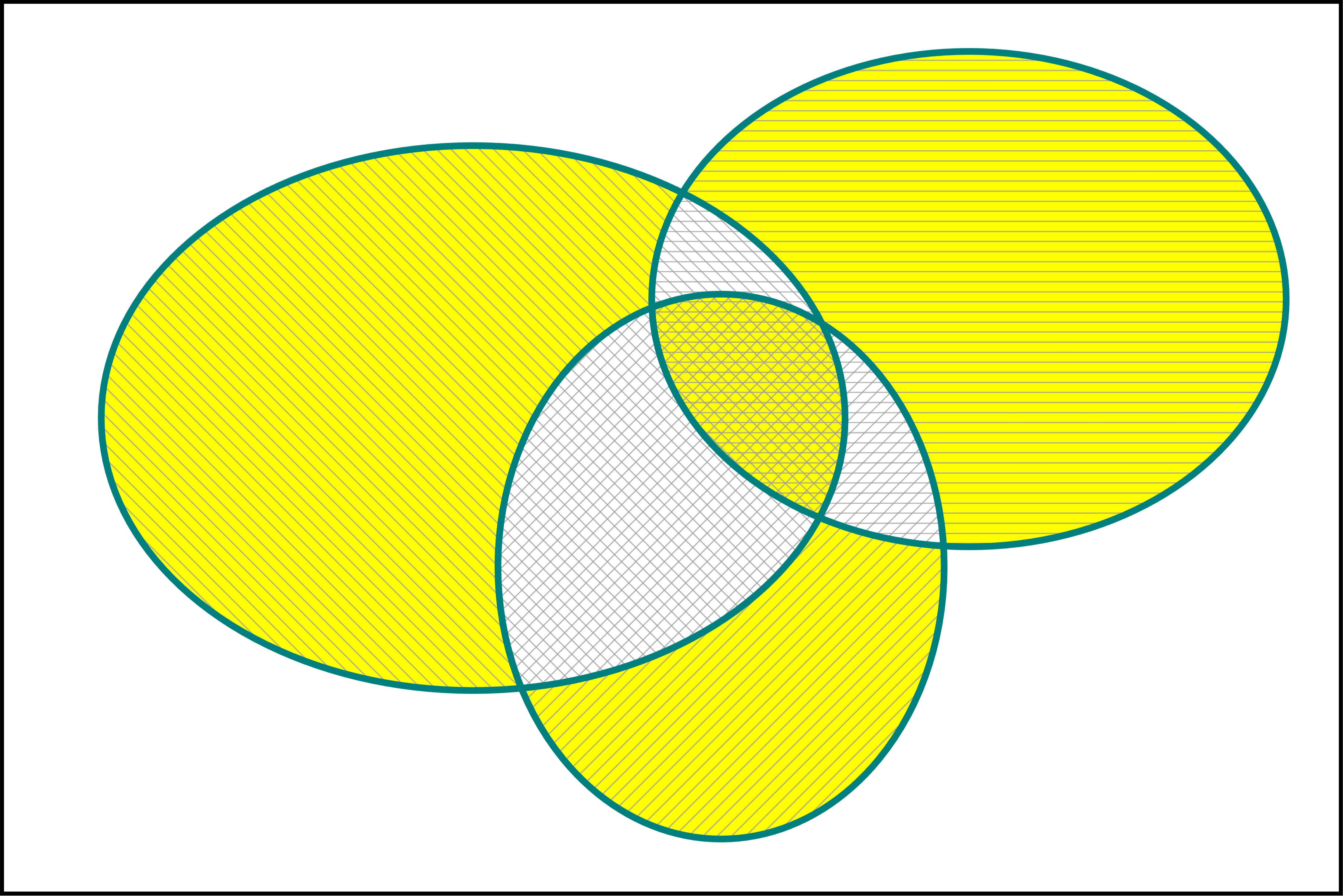
I updated the notes again today: The class lecture notes version of April 8, 2024 20:32. The only new item added is a Venn diagram of a three set symmetric difference, see Figure 10 on page 23. This picture was somewhat challenging to make, so I almost gave up. But, with some "brute force" I succeeded.
-
I vividly remember the fascination I felt when I was introduced to the set operation of symmetric difference of two sets in an undergraduate class on set theory. Let $A$ and $B$ be two sets. The symmetric difference of two sets $A$ and $B$, denoted by $A\Delta B$, is defined as \[ A\Delta B = ( A \setminus B ) \cup ( B \setminus A ). \] Here $A \setminus B$ and $B \setminus A$ are the set differences defined as \begin{align*} A \setminus B & = \bigl\{ x \in U : x \in A \land x \not\in B \bigr\}, \\ B \setminus A & = \bigl\{ x \in U : x \not\in A \land x \in B \bigr\}. \end{align*} Hence, in formal logical notation the symmetric difference of two sets operation is given as \[ A \Delta B = \Bigl\{ x \in U : \bigl( x \in A \land x \not\in B \bigr) \lor \bigl( x \not\in A \land x \in B \bigr) \Bigr\}. \] A different way of communicating the definition of the symmetric set difference is to give the following truth table. For arbitrary $x \in U$ we have the following four cases:
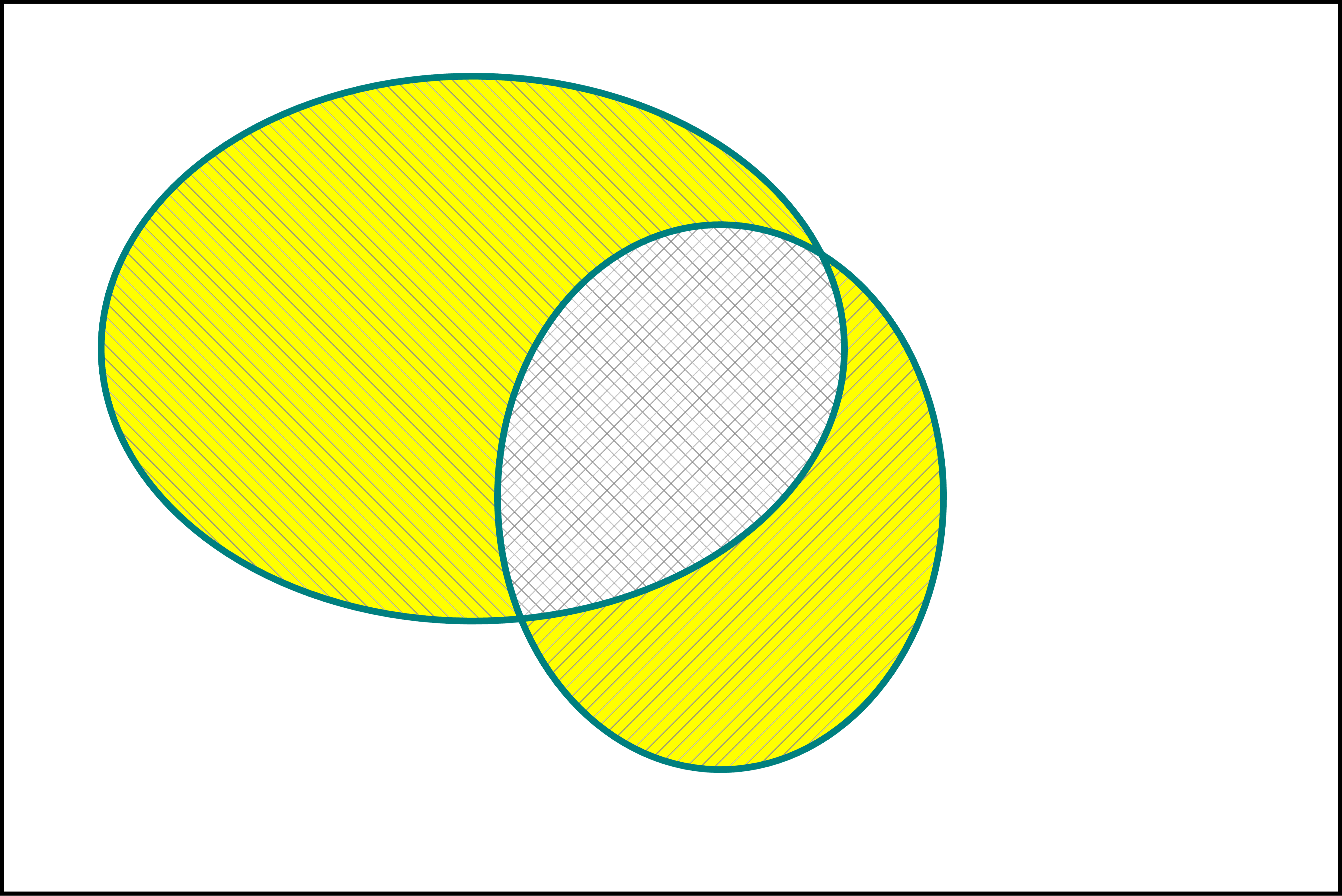
$x\in A$ $x\in B$ $x\in A\Delta B$ hatched F F F none F T T slope $1$ T F T slope $-1$ T T F slopes $-1$ and $1$ The above truth table is identical with the truth table of the EXCLUSIVE OR (XOR) compound proposition.
-
For interesting properties of the symmetric difference see it Wikipedia page.
Below is a Venn diagram of a symmetric difference of two sets $A$ and $B$. In the Venn diagram below, the set $A$ is hatched by thin grey lines with slope $-1$, and the set $B$ is hatched by thin grey lines with slope $1$.
A symmetric difference of two sets in yellow with a teal boundary
-
Below is a Venn diagram of a symmetric difference of three sets. In the Venn diagram below, the set $A$ is hatched by thin grey lines with slope $-1$, the set $B$ is hatched by thin grey lines with slope $1$, and the set $C$ is hatched by thin grey horizontal lines. The definition of the symmetric difference of three sets rests on the fact that the symmetric difference set operation $\Delta$ is associative: \[ (A \Delta B) \Delta C = A \Delta (B \Delta C) \] One way to prove the preceding equality is to set up the following truth table. For arbitrary $x \in U$ we have the following eight cases:
$x\in A$ $x\in B$ $x\in C$ $x\in A\Delta B$ $x\in (A\Delta B)\Delta C$ $x\in B\Delta C$ $x\in A\Delta (B\Delta C)$ hatched F F F F F F F none F F T F T T T slope $0$ F T F T T T T slope $1$ F T T T F F F slopes $1$, $0$ T F F T T F T slope $-1$ T F T T F T F slopes $-1$, $0$ T T F F F T F slopes $-1$, $1$ T T T F T F T slopes $-1$, $1$, $0$ The preceding truth table proves that the following proposition is true \[ \forall\mkern 1.5mu x \in U \qquad \Bigl( x\in (A\Delta B)\Delta C \ \ \Leftrightarrow \ \ x\in A\Delta (B\Delta C) \Bigr). \]
A symmetric difference of three sets in yellow with a teal boundary
- I am in the process of rewriting Section 3.2 Functions of Chapter Three on Sets and Functions. I am using my webpage Functions as a blueprint to rewrite this section.
- The information sheet
- In this class we present a rigorous approach to basic theorems in calculus. Since rigorous reasoning in Mathematics is based on Mathematical Logic, we will start with a Brief Review of Mathematical Logic. This is Chapter Two in the class lecture notes.
- Most, if not all mathematical statements, involve quantifiers. In the class lecture notes the quantifiers are presented in Section 2.3. Examples are given in Section 2.4. For additional examples, you can read my webpage Mathematical Rigor in the Context of Quadratic Functions.
- Some useful Wikipedia links:
- My one-page on the Power of Math. This page is a part of Chapter One in the class lecture notes.
- My one-page on Rigorous Reasoning. This page is a part of Chapter One in the class lecture notes.