- Minor rewriting of the The class lecture notes.
-
In today's post, I present a remarkable example of a proof using the Principle of Mathematical Induction. This proof is Example 4.5 in the book:
- Titu Andreescu, Vlad Crsan: Mathematical Induction: A Powerful and Elegant Method of Proof.
-
First recall the exact statement of the Principle of Mathematical Induction.
Principle of Mathematical Induction. By $\mathbb{N}$ we denote the set of positive integers. Let $P(n)$ be a propositional function with $n\in \mathbb{N}$. The following implication holds: \[ P(1) \land \Bigl( \forall \mkern 2mu k \in \mathbb{N} \ \ P(k) \Rightarrow P(k+1) \Bigr) \quad \Rightarrow \quad \forall \mkern 2mu n \in \mathbb{N} \ \ \ P(n) \]
- Let \(n \in \mathbb{N}\), and let \((a_1, \ldots, a_n) \in \mathbb{R}^n\). We will frequently refer to the sum and product of the components of such \(n\)-tuples. For this, we adopt the standard notation: \[ \prod_{i=1}^n a_i = a_1 \cdots a_n, \qquad \sum_{i=1}^n a_i = a_1 + \cdots + a_n. \] That is, the first expression denotes the product, and the second the sum, of the components of the \(n\)-tuple.
-
Statement of the problem from Andreescu-Crsan book:
Problem 1. Let $\mathbb{R}_{\gt 0}$ denote the set of all positive real numbers. For each $n \in \mathbb{N}$, let $\bigl(\mathbb{R}_{\gt 0}\bigr)^n$ denote the set of all $n$-tuples of positive real numbers. Prove that the following implication holds for all $n\in\mathbb{N}$: \[ \forall \mkern 2mu (a_1,\ldots,a_n) \in \bigl(\mathbb{R}_{\gt 0}\bigr)^n \qquad \prod_{i=1}^n a_i = 1 \quad \Rightarrow \quad \sum_{i=1}^n a_i \geq n . \] Equality in the last inequality holds if and only if $(a_1,\ldots,a_n) = (1,\ldots,1)$.
-
Proof of the inequality in Problem 1. (Proof by Mathematical Induction: The Base case and the Inductive step presented in five separate steps.)
- Let $n\in\mathbb{N}$. Denote by $P(n)$ the following statement: \[ \forall \mkern 1.5mu (a_1,\ldots,a_n) \in \bigl(\mathbb{R}_{\gt 0}\bigr)^n \qquad \bbox[4px, #88FF88, border: 2pt solid green]{\prod_{i=1}^n a_i = 1} \quad \Rightarrow \quad \bbox[4px, #FF7777, border: 2pt solid #990000]{\sum_{i=1}^n a_i \geq n}. \] We will use Mathematical Induction to prove: \[ \forall \mkern 1.5mu n\in\mathbb{N} \qquad P(n). \]
- Base case. The statement $P(1)$ reads: \[ \forall \mkern 1mu a_1 \in \mathbb{R}_{\gt 0} \qquad a_1 = 1 \quad \Rightarrow \quad a_1 = 1. \] The preceding implication is clearly true.
-
Inductive step. Let $k\in\mathbb{N}$ be arbitrary. We need to prove \[ \require{bbox} \bbox[4px, #88FF88, border: 2pt solid green]{P(k)} \quad \Rightarrow \quad \bbox[4px, #FF7777, border: 2pt solid #990000]{P(k+1)}. \] Assume $\bbox[4px, #88FF88, border: 2pt solid green]{P(k)}$. That is assume \[ \bbox[4px, #88FF88, border: 2pt solid green]{\forall \mkern 2mu (b_1,\ldots,b_k) \in \bigl(\mathbb{R}_{\gt 0}\bigr)^k \qquad \prod_{i=1}^k b_i = 1 \quad \Rightarrow \quad \sum_{i=1}^k b_i \geq k}. \] The preceding implication is the Inductive hypothesis.
We will prove $\bbox[4px, #FF7777, border: 2pt solid #990000]{P(k+1)}$. That is we will prove \[ \forall \mkern 2mu (a_1,\ldots,a_{k+1}) \in \bigl(\mathbb{R}_{\gt 0}\bigr)^{k+1} \qquad \bbox[4px, #88FF88, border: 2pt solid green]{\prod_{i=1}^{k+1} a_i = 1} \quad \Rightarrow \quad \bbox[4px, #FF7777, border: 2pt solid #990000]{\sum_{i=1}^{k+1} a_i \geq k+1}. \] Here is a proof of $\bbox[4px, #FF7777, border: 2pt solid #990000]{P(k+1)}$.
Step 1. Let $\bbox[4px, #88FF88, border: 2pt solid green]{(a_1,\ldots,a_{k+1}) \in \bigl(\mathbb{R}_{\gt 0}\bigr)^{k+1}}$ be arbitrary and assume \[ \bbox[4px, #88FF88, border: 2pt solid green]{\prod_{i=1}^{k+1} a_i = 1}. \] Since neither product, nor sum depend on the order of the $(k+1)$-tuple, we can also assume that \[ \bbox[4px, #88FF88, border: 2pt solid green]{ \forall \mkern 1mu i \in \{1,\ldots,k+1\} \quad a_1 \leq a_i \leq a_{k+1}}. \]
Step 2. The order assumed in the last green box and Axiom OT (the relation of order among real numbers is transitive), together yield the following implication: \[ \bbox[4px, #88FF88, border: 2pt solid green]{ a_{k+1} \lt 1} \quad \Rightarrow \quad \bbox[4px, #88FF88, border: 2pt solid green]{ \forall \mkern 1mu i \in \{1,\ldots,k+1\} \ \ a_i \lt 1} \quad \Rightarrow \quad \bbox[4px, #88FF88, border: 2pt solid green]{\prod_{i=1}^{k+1} a_i \lt 1}. \] Hence the following implication holds: \[ \bbox[4px, #88FF88, border: 2pt solid green]{a_{k+1} \lt 1 \quad \Rightarrow \quad \prod_{i=1}^{k+1} a_i \lt 1}. \] The contrapositive of this implication is \[ \bbox[4px, #88FF88, border: 2pt solid green]{ \prod_{i=1}^{k+1} a_i \geq 1 \quad \Rightarrow \quad a_{k+1} \geq 1}. \] Since we assume, \[ \bbox[4px, #88FF88, border: 2pt solid green]{\prod_{i=1}^{k+1} a_i = 1}, \] from the contrapositive, we deduce that $\bbox[4px, #88FF88, border: 2pt solid green]{a_{k+1} \geq 1}$.
Step 3. Similarly, the implication below follows from the order assumed in the green box before Step 2`: \[ \bbox[4px, #88FF88, border: 2pt solid green]{ a_{1} \gt 1 \quad \Rightarrow \quad \prod_{i=1}^{k+1} a_i \gt 1}. \] The contrapositive of the preceding implication is \[ \bbox[4px, #88FF88, border: 2pt solid green]{ \prod_{i=1}^{k+1} a_i \leq 1 \quad \Rightarrow \quad a_{1} \leq 1}. \] Since we assume \[ \bbox[4px, #88FF88, border: 2pt solid green]{\prod_{i=1}^{k+1} a_i = 1}, \] the contrapositive implies \[ \bbox[4px, #88FF88, border: 2pt solid green]{a_1 \leq 1}. \]
Step 4. In Step 2 and Step 3 we proved \(\bbox[4px, #88FF88, border: 2pt solid green]{a_1 \leq 1}\) and \(\bbox[4px, #88FF88, border: 2pt solid green]{a_{k+1} \geq 1}\). Consequently, \begin{equation*} \bbox[4px, #88FF88, border: 2pt solid green]{\bigl(1-a_1\bigr) \bigl(1-a_{k+1}\bigr) \leq 0}, \end{equation*} and therefore, \begin{equation*} \bbox[4px, #88FF88, border: 2pt solid green]{a_1 a_{k+1} \leq a_1 + a_{k+1} - 1}. \end{equation*}
Step 5. Now we use the Inductive hypothesis: \[ \bbox[4px, #88FF88, border: 2pt solid green]{\forall \mkern 2mu (b_1,\ldots,b_k) \in \bigl(\mathbb{R}_{\gt 0}\bigr)^k \qquad \prod_{i=1}^k b_i = 1 \quad \Rightarrow \quad \sum_{i=1}^k b_i \geq k}. \] To use the Inductive hypothesis we need to define a \(k\)-tuple $(b_1,\ldots,b_k)$. If \(k=1\), we set $(b_1) = (a_1a_{k+1})$. If \(k \gt 1\), let the elements of $(b_1,\ldots,b_k)$ be defined as follows \begin{equation*} \bbox[4px, #88FF88, border: 2pt solid green]{b_1 = a_1a_{k+1}, \quad b_i = a_i \quad \forall \mkern 1mu i \in \{2,\ldots,k\}}. \end{equation*} Recall that we assume \[ \bbox[4px, #88FF88, border: 2pt solid green]{\prod_{i=1}^{k+1} a_i = 1}. \] By the definition of $(b_1,\ldots,b_k)$ we have \[ \bbox[4px, #88FF88, border: 2pt solid green]{ \prod_{i=1}^k b_i = \prod_{i=1}^{k+1} a_i = 1}. \] Now we apply the Inductive hypothesis and deduce that \[ \bbox[4px, #88FF88, border: 2pt solid green]{ \sum_{i=1}^k b_i \geq k}. \] Recall that we proved \[ \bbox[4px, #88FF88, border: 2pt solid green]{b_1 = a_1 a_{k+1} \leq a_1 + a_{k+1} - 1}. \] Therefore \[ \bbox[4px, #88FF88, border: 2pt solid green]{ k \leq \sum_{i=1}^k b_i = a_1a_{k+1} + \sum_{i=2}^k a_i \leq a_1 + a_{k+1} - 1 + \sum_{i=2}^k a_i}. \] Consequently, \[ \bbox[4px, #88FF88, border: 2pt solid green]{k+1 \leq \sum_{i=1}^{k+1} a_i}, \quad \text{that is} \quad \bbox[4px, #88FF88, border: 2pt solid green]{\sum_{i=1}^{k+1} a_i \geq k+1}. \] This completes the proof of \(P(k+1)\).
-
To prove the necessary and sufficient condition for equality to hold in the inequality we have to prove the following implication.
For all $n\in\mathbb{N}$ and for all \((a_1,\ldots,a_n) \in \bigl(\mathbb{R}_{\gt 0}\bigr)^n\) the following implication holds \[ \prod_{i=1}^n a_i = 1 \ \land \ \sum_{i=1}^n a_i = n \quad \Rightarrow \quad (a_1,\ldots,a_n) = (1,\ldots,1). \]
-
Proof of the characterization of equality. (Proof by Mathematical Induction: the Base case and the Inductive step presented in three steps.)
- Let $n\in\mathbb{N}$. Denote by $P(n)$ the following statement: For all \((a_1,\ldots,a_n) \in \bigl(\mathbb{R}_{\gt 0}\bigr)^n\) the following implication holds \[ \bbox[4px, #88FF88, border: 2pt solid green]{\prod_{i=1}^n a_i = 1 \ \land \ \sum_{i=1}^n a_i = n} \quad \Rightarrow \quad \bbox[4px, #FF7777, border: 2pt solid #990000]{(a_1,\ldots,a_n) = (1,\ldots,1)}. \]
- Base case. The statement $P(1)$ reads: For all \(a_1 \in \mathbb{R}_{\gt 0}\) the following implication holds \[ \bbox[4px, #88FF88, border: 2pt solid green]{a_1 = 1 \ \land \ a_1 = 1} \quad \Rightarrow \quad \bbox[4px, #FF7777, border: 2pt solid #990000]{a_1 = 1}. \] The preceding implication is clearly true.
-
Inductive step. Let $k\in\mathbb{N}$ be arbitrary. We need to prove \[ \bbox[4px, #88FF88, border: 2pt solid green]{P(k)} \quad \Rightarrow \quad \bbox[4px, #FF7777, border: 2pt solid #990000]{P(k+1)}. \] Assume $P(k)$. That is assume: For all \((b_1,\ldots,b_k) \in \bigl(\mathbb{R}_{\gt 0}\bigr)^k\) the following implication holds \[ \bbox[4px, #88FF88, border: 2pt solid green]{\prod_{i=1}^k b_i = 1 \ \land \ \sum_{i=1}^k b_i = k \quad \Rightarrow \quad (b_1,\ldots,b_k) = (1,\ldots,1)}. \] The preceding implication is the Inductive hypothesis.
We will prove $\bbox[4px, #FF7777, border: 2pt solid #990000]{P(k+1)}$. That is we will prove: For all \((a_1,\ldots,a_{k+1}) \in \bigl(\mathbb{R}_{\gt 0}\bigr)^{k+1}\) the following implication holds \[ \bbox[4px, #88FF88, border: 2pt solid green]{\prod_{i=1}^{k+1} a_i = 1 \ \land \ \sum_{i=1}^{k+1} a_i = {k+1}} \quad \Rightarrow \quad \bbox[4px, #FF7777, border: 2pt solid #990000]{(a_1,\ldots,a_{k+1}) = (1,\ldots,1)}. \] Here is a proof of $\bbox[4px, #FF7777, border: 2pt solid #990000]{P(k+1)}$.
Step 6. Let $\bbox[4px, #88FF88, border: 2pt solid green]{(a_1,\ldots,a_{k+1}) \in \bigl(\mathbb{R}_{\gt 0}\bigr)^{k+1}}$ be arbitrary and assume \[ \bbox[4px, #88FF88, border: 2pt solid green]{ \prod_{i=1}^{k+1} a_i = 1 \ \land \ \sum_{i=1}^{k+1} a_i = {k+1}}. \] Since neither product, nor sum depend on the order of the $(k+1)$-tuple, we can also assume that \[ \bbox[4px, #88FF88, border: 2pt solid green]{ \forall \mkern 1mu i \in \{1,\ldots,k+1\} \quad a_1 \leq a_i \leq a_{k+1}}. \] In the same way as in Step 2 and Step 3 of the Proof of the inequality we can prove that \(\bbox[4px, #88FF88, border: 2pt solid green]{a_1 \leq 1}\) and \(\bbox[4px, #88FF88, border: 2pt solid green]{a_{k+1} \geq 1}\). Consequently, \begin{equation*} \bbox[4px, #88FF88, border: 2pt solid green]{\bigl(1-a_1\bigr) \bigl(1-a_{k+1}\bigr) \leq 0}, \end{equation*} and therefore, \begin{equation*} \bbox[4px, #88FF88, border: 2pt solid green]{ a_1 a_{k+1} \leq a_1 + a_{k+1} - 1}. \end{equation*}
Step 7. Now we use the Inductive hypothesis: \[ \bbox[4px, #88FF88, border: 2pt solid green]{\prod_{i=1}^k b_i = 1 \ \land \ \sum_{i=1}^k b_i = k \quad \Rightarrow \quad (b_1,\ldots,b_k) = (1,\ldots,1)}. \] To use the Inductive hypothesis we need to define a \(k\)-tuple $(b_1,\ldots,b_k)$. If \(k=1\), we set $(b_1) = (a_1a_{k+1})$. If \(k \gt 1\), let the elements of $(b_1,\ldots,b_k)$ be defined as follows \begin{equation*} \bbox[4px, #88FF88, border: 2pt solid green]{ b_1 = a_1a_{k+1}, \qquad b_i = a_i \quad \forall \mkern 1mu i \in \{2,\ldots,k\}}. \end{equation*} Then we have \[ \bbox[4px, #88FF88, border: 2pt solid green]{ \prod_{i=1}^k b_i = \prod_{i=1}^{k+1} a_i = 1}. \] To apply the Inductive hypothesis we need to prove \[ \bbox[4px, #FF7777, border: 2pt solid #990000]{ \sum_{i=1}^k b_i = k}. \] Let us prove this equality. We use the inequality \[ \bbox[4px, #88FF88, border: 2pt solid green]{ a_1 a_{k+1} \leq a_1 + a_{k+1} - 1}, \] which is proven in Step 6, and the assumption \[ \bbox[4px, #88FF88, border: 2pt solid green]{ \sum_{i=1}^{k+1} a_i = {k+1}}. \] The last two green boxes yield \begin{equation*} \bbox[4px, #88FF88, border: 2pt solid green]{ \sum_{i=1}^k b_i = a_1a_{k+1} + \sum_{i=2}^k a_i \leq \sum_{i=1}^{k+1} a_i - 1 = k}. \end{equation*} The following implication has been already proven in Problem 1: \[ \bbox[4px, #88FF88, border: 2pt solid green]{ \prod_{i=1}^k b_i = 1 \quad \Rightarrow \quad \sum_{i=1}^k b_i \geq k}. \] Since \[ \bbox[4px, #88FF88, border: 2pt solid green]{ \prod_{i=1}^k b_i = 1} \] is true, we deduce \[ \bbox[4px, #88FF88, border: 2pt solid green]{\sum_{i=1}^k b_i \geq k}. \] Thus we proved \[ \bbox[4px, #88FF88, border: 2pt solid green]{\sum_{i=1}^k b_i \leq k} \quad \text{and} \quad \bbox[4px, #88FF88, border: 2pt solid green]{\sum_{i=1}^k b_i \geq k}. \] Consequently, \[ \bbox[4px, #88FF88, border: 2pt solid green]{\sum_{i=1}^k b_i = k}. \] Since we proved \[ \bbox[4px, #88FF88, border: 2pt solid green]{ \prod_{i=1}^k b_i = 1 \ \land \ \sum_{i=1}^k b_i = k}, \] the Inductive hypothesis, \[ \bbox[4px, #88FF88, border: 2pt solid green]{ \prod_{i=1}^k b_i = 1 \ \land \ \sum_{i=1}^k b_i = k \quad \Rightarrow \quad \bigl(b_1,\ldots, b_k\bigr) = (1,\ldots,1)}, \] implies the equality \[ \bbox[4px, #88FF88, border: 2pt solid green]{ \bigl(b_1,\ldots, b_k\bigr) = (1,\ldots,1)}. \]
Step 8. Consequently, by the definition of the \(k\)-tuple \(\bigl(b_1,\ldots, b_k\bigr)\), we have \[ \bbox[4px, #88FF88, border: 2pt solid green]{ b_1 = a_1 a_{k+1} = 1 \quad \text{and} \quad b_i = a_i = 1 \ \ \forall \mkern 1.5mu i \in \{2,\ldots,k\}}. \] Recall that we assume \[ \bbox[4px, #88FF88, border: 2pt solid green]{ \sum_{i=1}^{k+1} a_i = k+1}, \] and we just proved for all \( i \in \{2,\ldots,k\}\) we have \(a_i = 1\). Therefore, \[ \bbox[4px, #88FF88, border: 2pt solid green]{ k+1 = \sum_{i=1}^{k+1} a_i = a_1 + \sum_{i=2}^{k} a_i + a_{k+1} = a_1 + (k-1) + a_{k+1}}. \] Consequently, \[ \bbox[4px, #88FF88, border: 2pt solid green]{a_1 + a_{k+1} = 2}. \] Hence, we have \[ \bbox[4px, #88FF88, border: 2pt solid green]{a_1 a_{k+1} = 1} \quad \text{and} \quad \bbox[4px, #88FF88, border: 2pt solid green]{a_1 + a_{k+1} = 2}. \] Since both \(a_1\) and \(a_{k+1}\) are positive multiplying the second equality by \(a_1\) and using the first equality, yields \(\bbox[4px, #88FF88, border: 2pt solid green]{a_1^2 + 1 = 2 a_1}\). That is, \[ \bbox[4px, #88FF88, border: 2pt solid green]{ 0 = a_1^2 + 1 - 2 a_1 = \bigl(a_1 - 1\bigr)^2}. \] Consequently, \(\bbox[4px, #88FF88, border: 2pt solid green]{a_1 = 1}\) and thus \(\bbox[4px, #88FF88, border: 2pt solid green]{a_{k+1}=1}\), since \(\bbox[4px, #88FF88, border: 2pt solid green]{a_1 a_{k+1} = 1}\). In conclusion, we proved \[ \bbox[4px, #88FF88, border: 2pt solid green]{ \bigl(a_1,\ldots, a_{k+1}\bigr) = (1,\ldots,1)}. \] This completes the Proof of the characterization of equality.
-
An application of the above problem provides one of the simplest proofs of the Inequality of Arithmetic and Geometric Means, see the Wikipedia page AM-GM Inequality
Proof of the AM-GM Inequality.AM-GM Inequality. Let $\mathbb{R}_{\gt 0}$ denote the set of all positive real numbers. For each $n \in \mathbb{N}$, let $\bigl(\mathbb{R}_{\gt 0}\bigr)^n$ denote the set of all $n$-tuples of positive real numbers. Prove that the following implication holds for all $n\in\mathbb{N}$: \[ \forall\mkern 2mu (x_1,\ldots,x_n) \in \bigl(\mathbb{R}_{\gt 0}\bigr)^n \qquad \sqrt[n]{x_1 \cdots x_n} \leq \frac{x_1 + \cdots + x_n}{n}. \] Equality in the last inequality holds if and only if $x_1 = \cdots = x_n$.
- Let $\bbox[4px, #88FF88, border: 2pt solid green]{n\in\mathbb{N}}$ and $\bbox[4px, #88FF88, border: 2pt solid green]{(x_1,\ldots,x_n) \in \bigl(\mathbb{R}_{\gt 0}\bigr)^n}$ be arbitrary. The objective is to prove that \[ \bbox[4px, #FF7777, border: 2pt solid #990000]{ \sqrt[n]{x_1 \cdots x_n} \leq \frac{x_1 + \cdots + x_n}{n}}. \] Define $\bbox[4px, #88FF88, border: 2pt solid green]{\alpha = \sqrt[n]{x_1 \cdots x_n}}$. Then $\bbox[4px, #88FF88, border: 2pt solid green]{\alpha \gt 0}$ and $\bbox[4px, #88FF88, border: 2pt solid green]{\alpha^n = x_1 \cdots x_n}$. Define \[ \forall\mkern 1mu i \in \{1,\ldots,n\} \quad \bbox[4px, #88FF88, border: 2pt solid green]{a_i = \frac{x_i}{\alpha}}. \] Then, \[ \bbox[4px, #88FF88, border: 2pt solid green]{ (a_1,\ldots,a_n) \in \bigl(\mathbb{R}_{\gt 0}\bigr)^n \ \ \land \ \ \prod_{i=1}^n a_i = \frac{x_1 \cdots x_n}{\alpha^n} = 1}. \] By the implication proved in Problem 1, we deduce that \[ \bbox[4px, #88FF88, border: 2pt solid green]{ n \leq \sum_{i=1}^n a_i = \frac{1}{\alpha}\bigl( x_1 + \cdots + x_n \bigr)}. \] Consequently, since $\bbox[4px, #88FF88, border: 2pt solid green]{n \gt 0}$ and $\bbox[4px, #88FF88, border: 2pt solid green]{\alpha \gt 0}$, we have \[ \bbox[4px, #88FF88, border: 2pt solid green]{ \sqrt[n]{x_1 \cdots x_n} = \alpha \leq \frac{1}{n}\bigl( x_1 + \cdots + x_n \bigr)}. \] Thus, the red box has been greenified. This completes the Proof of the AM-GM Inequality.
-
We started with Problem 1 which is a special case of the AM-GM Inequality, then we used Problem 1 to prove the AM-GM Inequality. We could have chosen a different special case of the AM-GM Inequality and formulated it as a problem. The proof is likely similar, though I have not carried it out myself. Therefore, it remains my conjecture for now.
Problem 2. Let $\mathbb{R}_{\gt 0}$ denote the set of all positive real numbers. For each $n \in \mathbb{N}$, let $\bigl(\mathbb{R}_{\gt 0}\bigr)^n$ denote the set of all $n$-tuples of positive real numbers. Prove that the following implication holds for all $n\in\mathbb{N}$: \[ \forall \mkern 2mu (a_1,\ldots,a_n) \in \bigl(\mathbb{R}_{\gt 0}\bigr)^n \qquad \sum_{i=1}^n a_i = n \quad \Rightarrow \quad \prod_{i=1}^n a_i \leq 1. \] Equality in the last inequality holds if and only if $(a_1,\ldots,a_n) = (1,\ldots,1)$.
Problem 2 in \(\mathbb{R}^2\) 
Problem 2 in \(\mathbb{R}^3\) In the figure with the caption "Problem 2 in \(\mathbb{R}^2\)" all points are in \(\bigl(\mathbb{R}_{\gt 0}\bigr)^2\). The points \((a_1,a_2) \in \bigl(\mathbb{R}_{\gt 0}\bigr)^2\) which satisfy \(a_1 a_2 = 1\) are represented by the solid orange hyperbola. The points satisfying \(a_1 a_2 \leq 1\) are represented by the light orange region. The points satisfying \(a_1 + a_2 = 2\) are represented by the solid blue line segment. So, the statement of Problem 2 reads: All the solid blue points are in the light orange region.
The characterization of the equality reads: The only point which is both orange and blue is \((1,1)\).
In the figure with the caption "Problem 2 in \(\mathbb{R}^3\)" all points are in \(\bigl(\mathbb{R}_{\gt 0}\bigr)^3\). The points \((a_1,a_2,a_3) \in \bigl(\mathbb{R}_{\gt 0}\bigr)^3\) which satisfy \(a_1 a_2 a_3 = 1\) are represented by the solid orange surface. The points satisfying \(a_1 a_2 a_3 \leq 1\) are represented by the light orange region. The points satisfying \(a_1 + a_2 + a_3 = 3\) are represented by the solid blue triangle. So, the statement of Problem 2 reads: All the solid blue points are in the light orange region.
The characterization of the equality reads: The only point which is both orange and blue is \((1,1,1)\).
In the figure with the caption "Problem 1 in \(\mathbb{R}^2\)" all points are in \(\bigl(\mathbb{R}_{\gt 0}\bigr)^2\). The points \((a_1,a_2) \in \bigl(\mathbb{R}_{\gt 0}\bigr)^2\) which satisfy \(a_1 a_2 = 1\) are represented by the solid orange hyperbola. The points satisfying \(a_1 + a_2 = 2\) are represented by the solid blue line segment. The points satisfying \(a_1 + a_2 \geq 2\) are represented by the light blue region. So, the statement of Problem 1 reads: All the solid orange points are in the light blue region.
The characterization of the equality reads: The only point which is both orange and blue is \((1,1)\).
In the figure with the caption "Problem 1 in \(\mathbb{R}^3\)" all points are in \(\bigl(\mathbb{R}_{\gt 0}\bigr)^3\). The points \((a_1,a_2,a_3) \in \bigl(\mathbb{R}_{\gt 0}\bigr)^3\) which satisfy \(a_1 a_2 a_3 = 1\) are represented by the solid orange surface. The points satisfying \(a_1 + a_2 + a_3 = 3\) are represented by the solid blue triangle. The points satisfying \(a_1 + a_2 + a_3 \geq 3\) are represented by the light blue region. So, the statement of Problem 1 reads: All the solid orange points are in the light blue region.
The characterization of the equality reads: The only point which is both orange and blue is \((1,1,1)\).
- Some improvements in The class lecture notes.
-
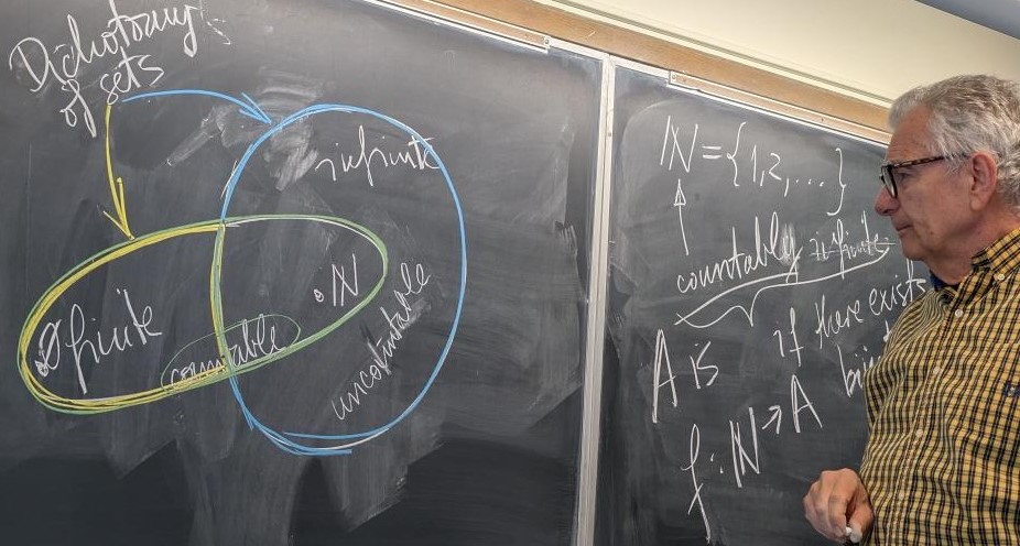
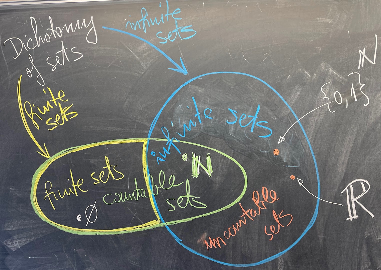
David took this picture of Me in Search of Set Terminology:
-
The terminology in the Venn diagram below is commonly used; however, in my notes, I propose a slightly different terminology.
-
Below is a ChatGPT-generated drawing of a child joyfully discovering a bijection between the fingers on their two hands.

-
Below is a baby looking for a bijection of the fingers on their two hands and discovering the same cardinality of two sets of fingers.

-
I return to the Triangle Inequality. Recall that the Triangle Inequality in \(\mathbb{R}\) is the following inequality: \[ \forall \mkern 1mu a, b \in \mathbb{R} \quad \text{we have} \quad |a+b| \leq |a|+|b|. \] Recall that the Reverse Triangle Inequality in \(\mathbb{R}\) is the following inequality: \[ \forall \mkern 1mu a, b \in \mathbb{R} \quad \text{we have} \quad \bigl| |a|-|b| \bigr| \leq |a-b|. \]
When working with an inequality, it is often helpful to rewrite it so that one side is greater than or equal to zero, which makes it easier to verify by plotting on a computer.
Thus, we rewrite the Triangle Inequality in the form \[ |a| + |b| - |a + b| \geq 0, \] and plot the left-hand side using graphing software. We expect the resulting graph to remain nonnegative, as illustrated in the figure below on the left. The graph is colored in shades between yellow and olive and confirms that the expression \(|a| + |b| - |a + b|\) is never negative over the domain we plotted.
Thus, we rewrite the Reverse Triangle Inequality in the form \[ |a-b| -\bigl| |a|-|b| \bigr| \geq 0 \] and plot the left-hand side using graphing software. We expect the resulting graph to remain nonnegative, as illustrated in the figure below on the right. The graph is colored in shades between cyan and teal and confirms that the expression \(|a-b| -\bigl| |a|-|b| \bigr|\) is never negative over the domain we plotted.
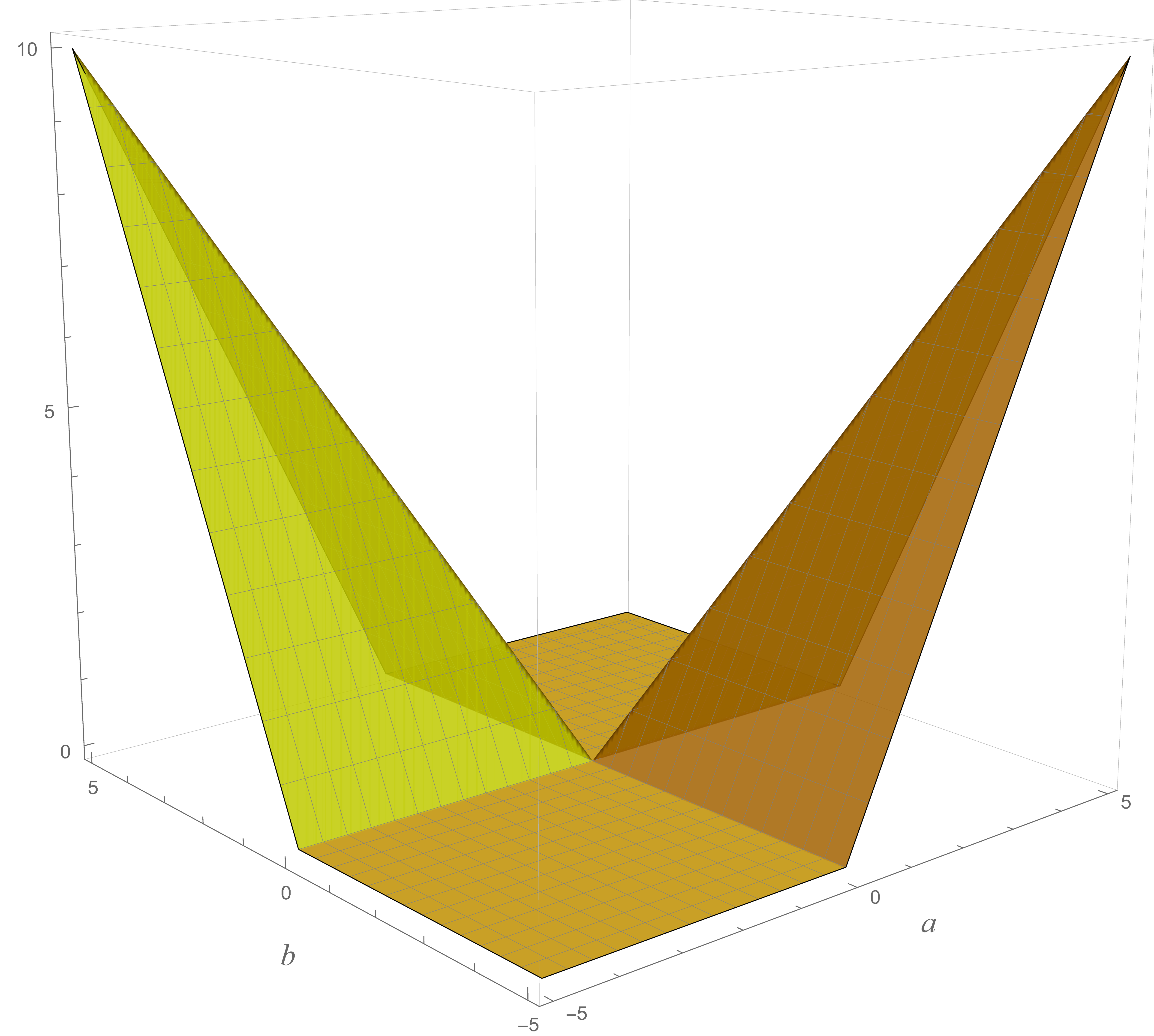
A plot of \(|a|+|b| - |a+b|\) 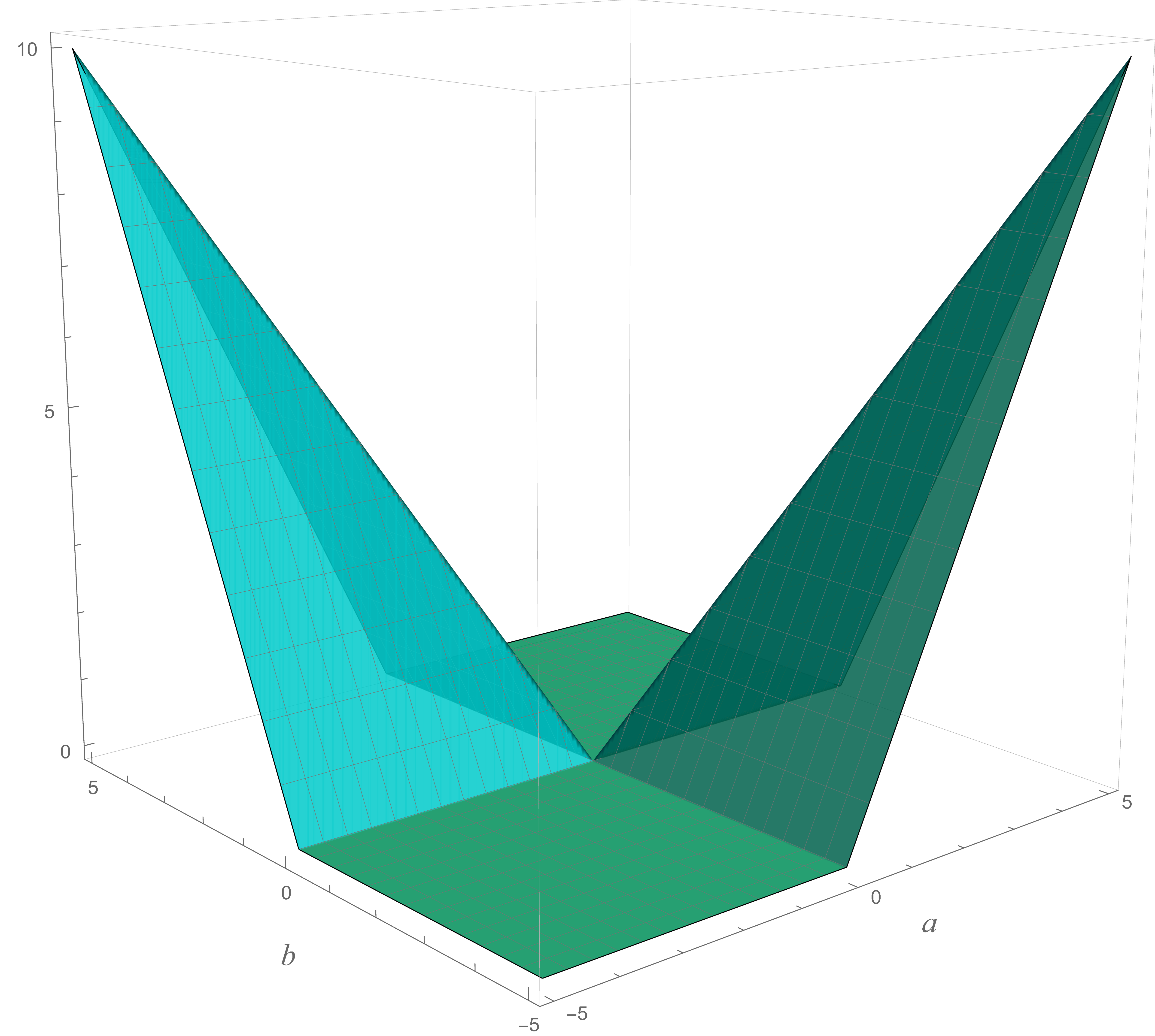
A plot of \(|a-b| -\bigl| |a|-|b| \bigr|\) The graphs reveal an additional insight: the dark yellow and dark cyan surfaces are identical, suggesting the following identity: \[ \forall \mkern 1mu a, b \in \mathbb{R} \quad \text{we have} \quad |a| + |b| - |a + b| = |a - b| - \bigl|\,|a| - |b|\,\bigr|. \] In this sense, the Triangle Inequality and the Reverse Triangle Inequality are essentially two expressions of the same underlying inequality.
We can verify this conjecture by plotting the difference \[ |a|+|b| - |a+b| - \bigl( |a-b| -\bigl| |a|-|b| \bigr| \bigr). \] And that is what we do in the figure below:
A plot of \(|a|+|b| - |a+b| - \bigl( |a-b| -\bigl| |a|-|b| \bigr| \bigr)\)
In the next item I prove the identity that we discovered in this item.
-
Theorem. Triangle Inequality and its Reverse. For all real numbers \(a, b \in \mathbb{R}\) we have \[ \underbrace{|a| + |b| - |a+b|}_{\text{Triangle Inequality}} = \underbrace{|a - b| - \bigl| |a| - |b| \bigr|}_{\text{Reverse Triangle Inequality}}. \tag{TI=RTI} \label{TI=RTI} \]
Case 1. \(a = 0\). In this case both the left-hand side and the right-hand side of \eqref{TI=RTI} evaluate to \(0\). Thus the equality holds.
Case 2. \(a \neq 0\). First we consider a special case \(a = 1\) and we set \(b = x\). Then \eqref{TI=RTI} becomes \[ 1 + |x| - |1+x| = |1 - x| - \bigl| 1 - |x| \bigr|. \tag{SC} \label{SC} \] If \(x \geq 0\), then both the left-hand side and the right-hand side of \eqref{SC} evaluate to \(0\). Thus the equality holds.
If \(x \lt 0\), then \(1-x \gt 0\), \(|x| = - x\) and the right-hand side evaluates to \[ |1 - x| - \bigl| 1 - |x| \bigr| = 1 - x - | 1 + x |. \] Similarly, the left-hand side of \eqref{SC} evaluates to \[ 1 + |x| - |1+x| = 1 - x - |1+x|. \] Since we obtained the same expression, \eqref{SC} is proved.
Now substitute \(\displaystyle x = \frac{b}{a}\) in \eqref{SC} to obtain that \[ 1 + \left| \frac{b}{a} \right| - \left| 1 + \frac{b}{a} \right| = \left| 1 - \frac{b}{a} \right| - \left| 1 - \left| \frac{b}{a} \right| \mkern 1mu \right|, \] holds for all \(b\in\mathbb{R}\) and all \(a\in\mathbb{R}\setminus\{0\}\). Next, we multiply the last equality by \(|a| \gt 0\) and use the multiplicative property of the absolute value function to obtain \[ |a| + |b| - |a+b| = |a - b| - \bigl| |a| - |b| \bigr|. \]
-
The proofs of the Triangle Inequality and the Reverse Triangle Inequality presented in the class lecture notes differ significantly. The proof of the Reverse Triangle Inequality relies essentially on the Triangle Inequality along with some clever algebraic manipulations. However, since we have just shown that these two inequalities are, in a certain sense, the same inequality, one might expect their proofs to follow a similar structure.
Below, we present proofs of the Triangle Inequality and the Reverse Triangle Inequality that are nearly identical in form.
-
Before presenting proofs, we list all the the most significant background knowledge that we use in the proof.
Background Knowledge is as follows.
As in the class lecture notes, we use the following notation \[ \mathbb{R}_{\geq 0} = \bigl\{ x \in \mathbb{R} : x \geq 0 \bigr\}. \]
BK1. For all \(x \in \mathbb{R}\) we have \(x \leq |x|\).
BK2. For all \(x \in \mathbb{R}\) we have \(|x| \geq 0\).
BK3. For all \(x \in \mathbb{R}\) we have \(|x|^2 = x^2\).
BK4. For all \(x, y \in \mathbb{R}_{\geq 0}\) the following equivalence holds \begin{equation*} x \leq y \quad \Leftrightarrow \quad x^2 \leq y^2. \end{equation*}
BK5. For all \(x, y \in \mathbb{R}\) the following multiplicative property of the absolute value holds \(|x y| = |x|\mkern 1mu |y|\).
-
Theorem. Triangle Inequality. For all real numbers \(a, b \in \mathbb{R}\) we have \[ |a+b| \leq |a| + |b|. \]
Let \(a, b \in \mathbb{R}\) be arbitrary. By BK2 and Axiom OA, we have \(|a+b| \geq 0\) and \(|a| + |b| \geq 0\). Therefore, the first of the following sequence of equivalences is a consequence of BK3. The remaining equivalences are justified in the accompanying boxed statements. \begin{align*} \require{bbox} |a+b| \leq |a| + |b| \quad &\Leftrightarrow \quad |a+b|^2 \leq \bigl(|a| + |b|\bigr)^2 \\ \bbox[#88FF88, 0px, border:3px solid #008800]{\text{BK3}} \quad & \Leftrightarrow \quad (a+b)^2 \leq \bigl(|a| + |b|\bigr)^2 \\ \bbox[#88FF88, 0px, border:3px solid #008800]{\text{Axioms DL, MC}} \quad & \Leftrightarrow \quad a^2+ 2 ab + b^2 \leq |a|^2 + 2 |a| \mkern 1mu |b| + |b|^2 \\ \bbox[#88FF88, 0px, border:3px solid #008800]{\text{BK3}} \quad & \Leftrightarrow \quad a^2+ 2 ab + b^2 \leq a^2 + 2 |a| \mkern 1mu |b| + b^2 \\ \bbox[#88FF88, 0px, border:3px solid #008800]{\text{Axioms AO, AC, AZ}} \quad & \Leftrightarrow \quad 2 ab \leq 2 |a| \mkern 1mu |b| \\ \bbox[#88FF88, 0px, border:3px solid #008800]{\text{BK5}} \quad & \Leftrightarrow \quad 2 ab \leq 2 |a b| \\ \bbox[#88FF88, 0px, border:3px solid #008800]{\text{Axioms OM and }1/2 \gt 0} \quad & \Leftrightarrow \quad ab \leq |a b| \end{align*} Since by BK1 the inequality \(ab \leq |a b| \) is true, the preceding sequence of inequalities proves the Triangle Inequality.
-
Theorem. Reverse Triangle Inequality. For all real numbers \(a, b \in \mathbb{R}\) we have \[ \bigl| |a| - |b| \bigr| \leq |a - b|. \]
Let \(a, b \in \mathbb{R}\) be arbitrary. By BK2 we have \(|a-b| \geq 0\) and \(\bigl| |a| - |b| \bigr| \geq 0\). Therefore, the first of the following sequence of equivalences is a consequence of BK3. The remaining equivalences are justified in the accompanying boxed statements. \begin{align*} \require{bbox} \bigl| |a| - |b| \bigr| \leq |a - b| \quad &\Leftrightarrow \quad \bigl| |a| - |b| \bigr|^2 \leq |a - b|^2 \\ \bbox[#88FF88, 0px, border:3px solid #008800]{\text{BK3}} \quad & \Leftrightarrow \quad \bigl( |a| - |b| \bigr)^2 \leq \bigl( a - b \bigr)^2 \\ \bbox[#88FF88, 0px, border:3px solid #008800]{\text{Axioms DL, MC}} \quad & \Leftrightarrow \quad |a|^2 - 2 |a|\mkern 1mu |b| + |b|^2 \leq a^2 - 2 ab + b^2 \\ \bbox[#88FF88, 0px, border:3px solid #008800]{\text{BK3 and BK5}} \quad & \Leftrightarrow \quad a^2 - 2 |ab| + b^2 \leq a^2 - 2 ab + b^2 \\ \bbox[#88FF88, 0px, border:3px solid #008800]{\text{Axioms AO, AC, AZ}} \quad & \Leftrightarrow \quad - 2 |ab| \leq - 2 ab \\ \bbox[#88FF88, 0px, border:3px solid #008800]{\text{Axioms OM and} 1/2 \gt 0} \quad & \Leftrightarrow \quad - |ab| \leq - ab \\ \bbox[#88FF88, 0px, border:3px solid #008800]{\text{Axioms OA, AO, AA}} \quad & \Leftrightarrow \quad ab \leq |ab| \end{align*} Since by BK1 the inequality \(ab \leq |a b| \) is true, the preceding sequence of inequalities proves the Reverse Triangle Inequality.
- A few small improvements: The class lecture notes.
-
In Subsection 4.3.2 Cardinality of intervals we construct a bijection between any two intervals of real numbers. See the details in the lecture notes. A bijection I find particularly cute is the following one: Its graph is symmetric, it is defined by an intriguing formula, and it is accompanied by an animation I created.
The function with domain \(\mathbb{R}_{\gt 0}\) and range \(\mathbb{R}_{\geq 0}\) given by the formula \[ \forall\mkern+0.5mu x \in \mathbb{R}_{\gt 0} \qquad x \mapsto 2 \lceil x \rceil - 1 - x, \] is a bijection. Its inverse is a function with domain \(\mathbb{R}_{\geq 0}\) and range \(\mathbb{R}_{\gt 0}\) is given by the formula: \[ \forall\mkern+0.5mu x \in \mathbb{R}_{\geq 0} \qquad x \mapsto 2 \lfloor x \rfloor + 1 - x. \] The claim that these two functions are inverses of each other is verified using properties of the floor and ceiling.
\(\forall\mkern+0.5mu x \in \mathbb{R}_{\gt 0} \quad x \mapsto 2 \lceil x \rceil - 1 - x\) 
\(\forall\mkern+0.5mu x \in \mathbb{R}_{\geq 0} \quad x \mapsto 2 \lfloor x \rfloor + 1 - x\) The animation below illustrates the action of the blue bijection above on the set of positive real numbers \(\mathbb{R}_{\gt 0}\). The set \(\mathbb{R}_{\gt 0}\) is split into half-open intervals \((n-1,n]\), where \(n \in \mathbb{N}\), the set of positive integers. Then, each of these intervals is flipped about its midpoint. That is the meaning of the blue plot above. The animation starts with the domain, \(\mathbb{R}_{\gt 0}\), the point \(0\) is excluded, signified by the circle placed on the number line at point corresponding to the number \(0\). The animation ends with the range, \(\mathbb{R}_{\geq 0}\), the point \(0\) is included, signified by the disk placed on the number line at the point corresponding to the number \(0\).
Place the cursor over the image to start the animation.

- The beautiful bijection from the preceding item with domain \(\mathbb{R}_{\gt 0}\) and range \(\mathbb{R}_{\geq 0}\) is discussed in the lecture notes in Remark 4.3.12.
-
The main bijection in the lecture notes in Subsection 4.3.2 Cardinality of intervals is the bijection \(\phi: \mathbb{R}_{\gt 0} \to \mathbb{R}_{\geq 0}\) given by the following piecewise formula \[ \forall\mkern+0.5mu x \in \mathbb{R}_{\gt 0} \qquad \phi(x) = \begin{cases} x & \text{if} \mkern+20mu x \in \mathbb{R}_{\gt 0} \setminus \mathbb{N}, \\[3pt] x - 1 & \text{if} \mkern+20mu x\in \mathbb{N}. \end{cases} \] Its inverse \[ \forall\mkern+0.5mu x \in \mathbb{R}_{\geq 0} \qquad \phi^{-1}(x) = \begin{cases} x & \text{if} \mkern+20mu x \in \mathbb{R}_{\gt 0} \setminus \mathbb{N}, \\[3pt] x + 1 & \text{if} \mkern+20mu x\in \mathbb{N}\cup\{0\}, \end{cases} \] is a bijection with domain \(\mathbb{R}_{\geq 0}\) and range \(\mathbb{R}_{\gt 0}\).
Here \[ \mathbb{N} = \bigl\{1,2,3,4, \ldots\bigr\} \] is the set of all positive integers.
Below is a graph of \(\phi: \mathbb{R}_{\gt 0} \to \mathbb{R}_{\geq 0}\) and its inverse \(\phi^{-1}: \mathbb{R}_{\geq 0} \to \mathbb{R}_{\gt 0}\).
The bijection \(\phi:\mathbb{R}_{\gt 0}\to \mathbb{R}_{\geq 0}\) 
The inverse \(\phi^{-1}:\mathbb{R}_{\geq 0}\to \mathbb{R}_{\gt 0}\) of the bijection \(\phi\) The animation below illustrates the action of the bijection \(\phi\) on the set of positive real numbers \(\mathbb{R}_{\gt 0}\). There is no action on the positive real numbers that are not positive integers. Positive integers are shifted backward. The animation ends with the range, \(\mathbb{R}_{\geq 0}\), the point \(0\) is included, signified by the disk placed on the number line at the point corresponding to the number \(0\).
Place the cursor over the image to start the animation.
- In today's post I will present an alternative proof of the Triangle Inequality and the Reverse Triangle Inequality.
-
Theorem. Triangle Inequality. For all real numbers \(a, b \in \mathbb{R}\) we have \[ |a+b| \leq |a| + |b|. \tag{TI1} \label{ti1} \] The equality holds in triangle equality \eqref{ti1} if and only if \(ab\geq 0\). Equivalently, the strict inequality holds in triangle equality \eqref{ti1} if and only if \(ab\lt 0\).
Let \(a,b \in \mathbb{R}\) be arbitrary. Consider two cases. Case 1. \(a = 0\). Then \eqref{ti1} becomes \(|b| = |b|\). Thus, in this case Triangle Inequality holds as an equality.
Case 2. \(a \neq 0\). Let us consider the special case \(a = 1\) first and set \(b=x\) where \(x\) is an arbitrary real number. That is prove: \[ |1+x| \leq 1 + |x|. \tag{TI2} \label{ti2} \] Let us look at two cases. If \(x \geq 0\), then \(1+x \gt 0\), and consequently \(|1+x| = 1 + x\) and \(1 + |x| = 1 + x\). Hence, in the case \(x \geq 0\), Triangle Inequality \eqref{ti2} holds as an equality. If \(x \lt 0\), then \(1 + |x| = 1- x\), and either \[ 1 + |x| - |1+x| = 1- x -(1+x) = -2 x \gt 0, \] or \[ 1 + |x| - |1+x| = 1- x -\bigl(-(1+x)\bigr) = 2 \gt 0. \] Thus, always \[ 1 + |x| - |1+x| \gt 0, \] that is, in the case \(x \lt 0\), Triangle Inequality \eqref{ti2} holds as a strict inequality.
Now substitute \(\displaystyle x = \frac{b}{a}\) in \eqref{ti2} to conclude that \[ \left| 1 + \frac{b}{a} \right| \leq 1 + \left| \frac{b}{a} \right| \] holds for all \(b\in\mathbb{R}\) and all \(a\in\mathbb{R}\setminus\{0\}\). Multiply the last equality by \(|a| \gt 0\) to get \[ |a|\mkern 1mu \left| 1 + \frac{b}{a} \right| \leq |a| + |a| \mkern 1mu\left| \frac{b}{a} \right|, \] By the multiplicative property of the absolute value function we have \[ |a|\mkern 1mu \left| 1 + \frac{b}{a} \right| = \left| a \left( 1 + \frac{b}{a} \right) \right| = | a + b | \] and \[ |a| \mkern 1mu\left| \frac{b}{a} \right| = | b |. \] Hence, the last inequality is the Triangle Inequality \eqref{ti1}: \[ |a+b| \leq |a| + |b|. \]
The case of strict inequality. Assume \(ab \lt 0\). Then \(a \neq 0\) and \(\displaystyle x = \frac{b}{a} \lt 0\). Therefore, the strict inequlity holds in \eqref{ti2}, and hence the strict inequality holds in Triangle Inequality \eqref{ti1}. Conversely, assume that the strict inequality holds in Triangle Inequality \eqref{ti1}. Then \(a\neq 0\). Dividing \eqref{ti1} by \(|a| \gt 0\), we conclude that the strict inequality holds in \eqref{ti2} with \(\displaystyle x = \frac{b}{a}\). Thus \(\frac{b}{a} \lt 0\). Multiplying by \(a^2 \gt 0\), we deduce that \(ab \lt 0\).
-
Theorem. Reverse Triangle Inequality. For all real numbers \(a, b \in \mathbb{R}\) we have \[ \bigl| |a| - |b| \bigr| \leq |a - b|. \tag{RTI1} \label{rti1} \] The equality holds in reverse triangle equality \eqref{rti1} if and only if \(ab\geq 0\). Equivalently, the strict inequality holds in triangle equality \eqref{rti1} if and only if \(ab\lt 0\).
I will present a strange proof. I will prove that in some sense the Triangle Inequality and the Reverse Triangle Inequality is the same inequality. For all \(a, b \in \mathbb{R}\) we have \[ |a - b| - \bigl| |a| - |b| \bigr| = |a| + |b| - |a+b|. \tag{RTI2} \label{rti2} \] For the proof we consider two cases.
Case 1. \(a = 0\). In this case both the left-hand side and the right-hand side of \eqref{rti2} evaluate to \(0\). Thus the equality holds.
Case 2. \(a \neq 0\). First we consider a special case \(a = 1\) and we set \(b = x\). Then \eqref{rti2} becomes \[ |1 - x| - \bigl| 1 - |x| \bigr| = 1 + |x| - |1+x|. \tag{RTI3} \label{rti3} \] If \(x \geq 0\), then both the left-hand side and the right-hand side of \eqref{rti3} evaluate to \(0\). Thus the equality holds.
If \(x \lt 0\), then \(1-x \gt 0\), \(|x| = - x\) and the left-hand side evaluates to \[ |1 - x| - \bigl| 1 - |x| \bigr| = 1 - x - | 1 + x |. \] Similarly, the right-hand side of \eqref{rti3} evaluates to \[ 1 + |x| - |1+x| = 1 - x - |1+x|. \] Since we obtained the same expression, \eqref{rti3} is proved.
Now substitute \(\displaystyle x = \frac{b}{a}\) in \eqref{rti3} to obtain that \[ \left| 1 - \frac{b}{a} \right| - \left| 1 - \left| \frac{b}{a} \right| \mkern 1mu \right| = 1 + \left| \frac{b}{a} \right| - \left| 1 + \frac{b}{a} \right|, \] holds for all \(b\in\mathbb{R}\) and all \(a\in\mathbb{R}\setminus\{0\}\). Next, we multiply the last inequality by \(|a| \gt 0\) and use the multiplicative property of the absolute value function to obtain \[ |a - b| - \bigl| |a| - |b| \bigr| = |a| + |b| - |a+b|. \]
The Reverse Triangle Inequality and its characterization of the equality now follows from the Triangle Inequality and its characterization of the equality.
- I added the identity function as one example of an important function on \(\mathbb{R}\) to Section 4.2 Five function to start with in the class lecture notes.
- I made many small improvements in Section 4.1 Axioms of the set \(\mathbb{R}\) in the class lecture notes.
- Today we discussed Cantor's theorem, Theorem 3.2.25 and talked about cardinality of infinite sets. That would complete Chapter Three on Sets and Functions.
-
In class I proved
Proposition 3.2.17. For an arbitrary nonempty set $S$ there exist a bijection between the power set of $S$ and the set $\{0,1\}^S$.
The table below illustrates the proof. Consider $S=\{\blacktriangle,\diamond,\bullet,\star\}$. The table below indicates what the bijection should be. The top part of the table contains sixteen functions in $\{0,1\}^S$; the bottom part contains the subsets of $A$ that are related to the functions above them.
$f_1$ $f_2$ $f_3$ $f_4$ $f_5$ $f_6$ $f_7$ $f_8$ $f_9$ $f_{10}$ $f_{11}$ $f_{12}$ $f_{13}$ $f_{14}$ $f_{15}$ $f_{16}$ $\blacktriangle$ $0$ $0$ $0$ $0$ $0$ $0$ $0$ $0$ $1$ $1$ $1$ $1$ $1$ $1$ $1$ $1$ $\diamond$ $0$ $0$ $0$ $0$ $1$ $1$ $1$ $1$ $0$ $0$ $0$ $0$ $1$ $1$ $1$ $1$ $\bullet$ $0$ $0$ $1$ $1$ $0$ $0$ $1$ $1$ $0$ $0$ $1$ $1$ $0$ $0$ $1$ $1$ $\star$ $0$ $1$ $0$ $1$ $0$ $1$ $0$ $1$ $0$ $1$ $0$ $1$ $0$ $1$ $0$ $1$ s u b s e t$\emptyset$ $\{\star\}$ $\{\bullet\}$ $\left\{\begin{array}{c}\!\!\bullet\!\!\\\!\!\star\!\! \end{array}\right\}$ $\{\diamond\}$ $\left\{\begin{array}{c}\!\!\diamond\!\!\\\!\!\star\!\!\end{array}\right\}$ $\left\{\begin{array}{c}\!\!\diamond\!\!\\\!\!\bullet\!\!\end{array}\right\}$ $\left\{\begin{array}{c}\!\!\diamond\!\!\\\!\!\bullet\!\!\\\!\!\star\!\! \end{array}\right\}$ $\{\blacktriangle\}$ $\left\{\begin{array}{c}\!\!\blacktriangle\!\!\\\!\!\star\!\!\end{array}\right\}$ $\left\{\begin{array}{c}\!\!\blacktriangle\!\!\\\!\!\bullet\!\! \end{array}\right\}$ $\left\{\begin{array}{c}\!\!\blacktriangle\!\!\\\!\!\bullet\!\!\\\!\!\star\!\! \end{array}\right\}$ $\left\{\begin{array}{c}\!\!\blacktriangle\!\!\\\!\!\diamond\!\! \end{array}\right\}$ $\left\{\begin{array}{c}\!\!\blacktriangle\!\!\\\!\!\diamond\!\!\\\!\!\star\!\! \end{array}\right\}$ $\left\{\begin{array}{c}\!\!\blacktriangle\!\!\\\!\!\diamond\!\!\\\!\!\bullet\!\! \end{array}\right\}$ $\left\{\begin{array}{c}\!\!\blacktriangle\!\!\\\!\!\diamond\!\!\\\!\!\bullet\!\!\\\!\!\star\!\! \end{array}\right\}$ The function \[ \Phi: \mathcal{P}(S) \to \{0,1\}^S \] defined in the proof of Proposition 3.2.17 is given in the columns of the above table. For example, in the above table, if $A = \{\blacktriangle,\bullet,\star\}$, then $\Phi(A) = f_{12}$, that is the function \[ f_{12}(\blacktriangle)=1, \quad f_{12}(\diamond)=0, \quad f_{12}(\bullet)=1, \quad f_{12}(\star)=1. \]
-
Recall Cantor's Theorem, that is Theorem 3.2.25 in the lecture notes:
Cantor's Theorem. Let $S$ be a nonempty set. Then there is no surjection with domain $S$ and codomain $\mathcal{P}(S)$.
In the proof of this theorem we prove \[ \forall\mkern+1.2mu \Theta: S \to \mathcal{P}(S) \quad \exists\mkern+1.5mu A \subseteq S \quad \forall\mkern+1.2mu x \in S \quad \Theta(x) \neq A. \] To prove the preceding displayed statement, let $\Theta: S \to \mathcal{P}(S)$ be an arbitrary function with domain \(S\) and codomain \(\mathcal{P}(S)\). To prove that $\Theta$ is not a surjection, we need to discover a subset $A$ of $S$ such that \[ \forall\mkern+1.2mu x \in S \quad \Theta(x) \neq A. \] The definition of such subset $A$ is truly ingenious, due to Georg Cantor: \[ A = \bigl\{ s \in S : s \not\in \Theta(s) \bigr\}. \]
-
I want to illustrate the universality of the definition of \(A\) on the example considered in the preceding item. Let \[ S=\{\blacktriangle,\diamond,\bullet,\star\}. \]
-
Next, I need to select a function \(\Theta: S \to \mathcal{P}(S)\). I randomly choose:
\[
\Theta(\blacktriangle) = \{\blacktriangle,\star\}, \quad
\Theta(\diamond) =\{\bullet,\star\} , \quad
\Theta(\bullet) = \{\blacktriangle,\bullet\}, \quad
\Theta(\star) = \{\bullet\}.
\]
Now, I construct the set \(A\), by asking:
- Is \(\blacktriangle \in A\)? That is, is \(\blacktriangle \in \Theta(\blacktriangle)\)? Yes. Thus, \(\blacktriangle \not\in A\)?
- Is \(\diamond \in A\)? That is, is \(\diamond \in \Theta(\diamond)\)? No. Thus, \(\diamond \in A\)?
- Is \(\bullet \in A\)? That is, is \(\bullet \in \Theta(\bullet)\)? Yes. Thus, \(\bullet \not\in A\)?
- Is \(\star \in A\)? That is, is \(\star \in \Theta(\star)\)? No. Thus, \(\star \in A\)?
-
Now I select a different function \(\Theta: S \to \mathcal{P}(S)\). I randomly choose:
\[
\Theta(\blacktriangle) = \{\blacktriangle,\diamond,\star\}, \quad
\Theta(\diamond) =\{\blacktriangle,\diamond,\bullet\} , \quad
\Theta(\bullet) = \{\star\}, \quad
\Theta(\star) = \{\blacktriangle, \star \}.
\]
Now, I construct the set \(A\), by asking:
- Is \(\blacktriangle \in A\)? That is, is \(\blacktriangle \in \Theta(\blacktriangle)\)? Yes. Thus, \(\blacktriangle \not\in A\)?
- Is \(\diamond \in A\)? That is, is \(\diamond \in \Theta(\diamond)\)? Yes. Thus, \(\diamond \not\in A\)?
- Is \(\bullet \in A\)? That is, is \(\bullet \in \Theta(\bullet)\)? No. Thus, \(\bullet \in A\)?
- Is \(\star \in A\)? That is, is \(\star \in \Theta(\star)\)? Yes. Thus, \(\star \not\in A\)?
- Two specific examples show the universality of the definition of \(A\). And, in the proof of Theorem 3.2.25 in the lecture notes, we demonstrated the for arbitrary nonempty set \(S\) and arbitrary \(\Theta: S \to \mathcal{P}(S)\), with \(A \subset S\) defined as \[ A = \bigl\{ s \in S : s \not\in \Theta(s) \bigr\}, \] we have \[ \forall\mkern+1.2mu x \in S \quad \Theta(x) \neq A. \]
- For a finite set \(S\) with \(n\) elements, the set \(\mathcal{P}(S)\) has \(2^n\) elements. Since for all \(n \in \mathbb{N}\) we have \(n \lt 2^n\), we could pursue a counting type proof that no surjection exists with domain \(S\) and codomain \(\mathcal{P}(S)\). But, for infinite sets, it is not clear that no such surjection exists.
- Using the concept of cardinality of sets, we proved that for every nonempty set \(S\) the cardinality of \(S\) is strictly smaller that the cardinality of \(\mathcal{P}(S)\). See Theorem 3.3.5 in the lecture notes, which is another version of Cantor's Theorem.
-
-
David took this picture of Cantor and Me:
- A handour that might help you deepen your understanding of Cantor's Theorem. If you want to practice Cantor's Algorithm used in the proof of Cantor's Theorem, you can print this blank table and experiment with different functions from \(S\) to \(\mathcal{P}(S)\) and algorithmically show that none of them is a surjection.
- I keep making small changes in class lecture notes.
-
The objective here is to prove that for an arbitrary nonempty set $S$ there exist a bijection between the power set of $S$ and the set $\{0,1\}^S$. Recall that $\{0,1\}^S$ denotes the set of all functions with domain \(S\) and codomain \(\{0,1\}\). Before presenting a formal proof, it is a good idea to consider an example. Consider $S=\{\blacktriangle,\diamond,\bullet,\star\}$. The table below indicates what the bijection should be. The top part of the table contains sixteen functions in $\{0,1\}^S$; the bottom part of the table contains the subsets of $S$ that are related to the functions above them.
$f_1$ $f_2$ $f_3$ $f_4$ $f_5$ $f_6$ $f_7$ $f_8$ $f_9$ $f_{10}$ $f_{11}$ $f_{12}$ $f_{13}$ $f_{14}$ $f_{15}$ $f_{16}$ $\blacktriangle$ $0$ $0$ $0$ $0$ $0$ $0$ $0$ $0$ $1$ $1$ $1$ $1$ $1$ $1$ $1$ $1$ $\diamond$ $0$ $0$ $0$ $0$ $1$ $1$ $1$ $1$ $0$ $0$ $0$ $0$ $1$ $1$ $1$ $1$ $\bullet$ $0$ $0$ $1$ $1$ $0$ $0$ $1$ $1$ $0$ $0$ $1$ $1$ $0$ $0$ $1$ $1$ $\star$ $0$ $1$ $0$ $1$ $0$ $1$ $0$ $1$ $0$ $1$ $0$ $1$ $0$ $1$ $0$ $1$ s u b s e t$\emptyset$ $\{\star\}$ $\{\bullet\}$ $\left\{\begin{array}{c}\!\!\bullet\!\!\\\!\!\star\!\! \end{array}\right\}$ $\{\diamond\}$ $\left\{\begin{array}{c}\!\!\diamond\!\!\\\!\!\star\!\!\end{array}\right\}$ $\left\{\begin{array}{c}\!\!\diamond\!\!\\\!\!\bullet\!\!\end{array}\right\}$ $\left\{\begin{array}{c}\!\!\diamond\!\!\\\!\!\bullet\!\!\\\!\!\star\!\! \end{array}\right\}$ $\{\blacktriangle\}$ $\left\{\begin{array}{c}\!\!\blacktriangle\!\!\\\!\!\star\!\!\end{array}\right\}$ $\left\{\begin{array}{c}\!\!\blacktriangle\!\!\\\!\!\bullet\!\! \end{array}\right\}$ $\left\{\begin{array}{c}\!\!\blacktriangle\!\!\\\!\!\bullet\!\!\\\!\!\star\!\! \end{array}\right\}$ $\left\{\begin{array}{c}\!\!\blacktriangle\!\!\\\!\!\diamond\!\! \end{array}\right\}$ $\left\{\begin{array}{c}\!\!\blacktriangle\!\!\\\!\!\diamond\!\!\\\!\!\star\!\! \end{array}\right\}$ $\left\{\begin{array}{c}\!\!\blacktriangle\!\!\\\!\!\diamond\!\!\\\!\!\bullet\!\! \end{array}\right\}$ $\left\{\begin{array}{c}\!\!\blacktriangle\!\!\\\!\!\diamond\!\!\\\!\!\bullet\!\!\\\!\!\star\!\! \end{array}\right\}$ How to read the above table? The top part of the table lists all the functions with domain $S=\{\blacktriangle,\diamond,\bullet,\star\}$ and codomain \(\{0,1\}\). For example, the function \(f_{12} : S\to \{0,1\}\) is the following function \[ f_{12}(\blacktriangle)=1, \quad f_{12}(\diamond)=0, \quad f_{12}(\bullet)=1, \quad f_{12}(\star)=1. \] In the bottom part of the table, below the function \(f_{12}\) you can find the subset $\{\blacktriangle,\bullet,\star\}$ of \(S = \{\blacktriangle,\diamond,\bullet,\star\}\).
Is there a relationship between the function \(f_{12}\) and the subset $\{\blacktriangle,\bullet,\star\}$?
This relationship is the key for the proof of Proposition 3.2.22 in the class notes. A more detailed proof of this proposition is given below in this post.
-
Definition. Let $S$ be a nonempty set and let \(A \subseteq S\). The function \({\large \chi}_{_{\mkern -3mu \Large A}}\mkern -4mu: S \to \{0,1\}\) defined by \[ \forall \mkern 1mu x \in S \qquad {\large \chi}_{_{\mkern -3mu \Large A}}\mkern-3mu(x) = \begin{cases} 1 & \text{if} \quad x \in A \\[5pt] 0 & \text{if} \quad x \in S\setminus A \end{cases} \] is called the indicator function of \(A\) relative to \(S\).
In the next two lemmas, I present two properties of indicator functions. The proofs of these lemmas are straightforward, but I include detailed proofs to illustrate how reasoning proceeds even in the most straightforward cases.
Lemma 1. Let \(S\) be a nonempty set, \(A\subseteq S\) and let \({\large \chi}_{_{\mkern -3mu \Large A}}:S\to \{0,1\}\) be the indicator function for \(A\). Then \[ \forall \mkern 1mu x \in S \qquad {\large \chi}_{_{\mkern -3mu \Large A}}\mkern-3mu(x) = 1 \quad \Leftrightarrow \quad x \in A. \]
The statement \[ \forall \mkern 1mu x \in S \qquad {\large \chi}_{_{\mkern -3mu \Large A}}\mkern-3mu(x) = 1 \quad \Leftrightarrow \quad x \in A \] involves a universal quantifier. To prove a statement that involves a universal quantifier, we begin by letting the quantified element be arbitrary. So, let \(x \in S\) be arbitrary.
Part 1. The implication \[ x \in A \quad \Rightarrow \quad {\large \chi}_{_{\mkern -3mu \Large A}}\mkern-3mu(x) = 1 \] follows from the first line in the definition of \({\large \chi}_{_{\mkern -3mu \Large A}}\) which says "if \(x\in A\), then \({\large \chi}_{_{\mkern -3mu \Large A}}\mkern-3mu(x) = 1\)."
Part 2. The implication \[ {\large \chi}_{_{\mkern -3mu \Large A}}\mkern-3mu(x) = 1 \quad \Rightarrow \quad x \in A \] follows from the second line in the definition of \({\large \chi}_{_{\mkern -3mu \Large A}}\) which says "if \(x\notin A\), then \({\large \chi}_{_{\mkern -3mu \Large A}}\mkern-3mu(x) = 0\)." The contrapositive of this implication from the definition is \[ {\large \chi}_{_{\mkern -3mu \Large A}}\mkern-3mu(x) \ne 0 \quad \Rightarrow \quad x \in A. \] However, since \({\large \chi}_{_{\mkern -3mu \Large A}}\mkern-3mu(x) \in \{0,1\}\), we have \[ {\large \chi}_{_{\mkern -3mu \Large A}}\mkern-3mu(x) = 1 \ \lor \ {\large \chi}_{_{\mkern -3mu \Large A}}\mkern-3mu(x) = 0. \] Therefore, by disjunctive syllogism, we deduce \[ {\large \chi}_{_{\mkern -3mu \Large A}}\mkern-3mu(x) \ne 0 \quad \Leftrightarrow \quad {\large \chi}_{_{\mkern -3mu \Large A}}\mkern-3mu(x) = 1. \] Hence, the implication from the second line in the definition of \({\large \chi}_{_{\mkern -3mu \Large A}}\) is equivalent to \[ {\large \chi}_{_{\mkern -3mu \Large A}}\mkern-3mu(x) = 1 \quad \Rightarrow \quad x \in A. \]
Since \(x\in S\) was arbitrary, we proved \[ \forall \mkern 1mu x \in S \qquad {\large \chi}_{_{\mkern -3mu \Large A}}\mkern-3mu(x) = 1 \quad \Leftrightarrow \quad x \in A. \] -
It is common to end a mathematical proof with a symbol. In some texts, the symbol ■ is used instead. In some texts, the proofs end with ■. Others use QED, short for the Latin phrase quod erat demonstrandum, meaning “that which was to be demonstrated.” On this webpage, I use a custom design QED that combines the black square ■ with the abbreviation QED.
-
Lemma 2. Let \(S\) be a nonempty set. For every \(f \in \{0,1\}^{\large S}\) there exists \(A\subseteq S\) such that \(f = {\large \chi}_{_{\mkern -3mu \Large A}}\).
Let \(f: S \to \{0,1\}\) be arbitrary. Set \[ A = \bigl\{ x\in S : f(x) = 1 \bigr\}. \] Next we prove \(f = {\large \chi}_{_{\mkern -3mu \Large A}}\). That is, we must prove \[ \forall \mkern 1mu x \in S \qquad f(x) = {\large \chi}_{_{\mkern -3mu \Large A}}\mkern-3mu(x). \] Let \(x\in S\) be arbitrary. Since \(f: S \to \{0,1\}\) we have two exclusive cases. Case 1: \(f(x) = 1\). By the definition of \(A\), in this case we have \(x\in A\). Therefore, \({\large \chi}_{_{\mkern -3mu \Large A}}\mkern-3mu(x) = 1\), and hence \(f(x) = {\large \chi}_{_{\mkern -3mu \Large A}}\mkern-3mu(x)\). Case 2: \(f(x) = 0\). In this case \(x\notin A\). Therefore, \({\large \chi}_{_{\mkern -3mu \Large A}}\mkern-3mu(x) = 0\), and hence \(f(x) = {\large \chi}_{_{\mkern -3mu \Large A}}\mkern-3mu(x)\). Thus, in each case \(f(x) = {\large \chi}_{_{\mkern -3mu \Large A}}\mkern-3mu(x)\). Since \(x\in S\) was arbitrary, we have proved \[ \forall \mkern 1mu x \in S \qquad f(x) = {\large \chi}_{_{\mkern -3mu \Large A}}\mkern-3mu(x). \]
- In the next item, I give a more detailed proof of Proposition 3.2.22 in the class notes. The proof of the proposition in the next item is inspired by the table in the first item in today's post. Below, by \(\mathcal{P}(S)\) we denote the power set, that is the family of all the subsets of a set \(S\).
-
Proposition 3.2.22. Let $S$ be a nonempty set. The function \(\Phi: \mathcal{P}(S) \to \{0,1\}^S\) defined by \[ \forall\mkern 1mu A \in \mathcal{P}(S) \qquad \Phi(A) = {\large \chi}_{_{\mkern -3mu \Large A}} \] is a bijection.
In Theorem 3.2.17 in the class notes we proved that a function is a bijection if and only if it is invertible. In this proof, we will prove that the function \(\Phi: \mathcal{P}(S) \to \{0,1\}^S\) defined in the proposition is invertible by defining its inverse.
To get inspiration for the definition of the inverse of \(\Phi: \mathcal{P}(S) \to \{0,1\}^S\) we look at the table in the first item in today's post. Ask yourself: where in the table do we see the function \(\Phi: \mathcal{P}(S) \to \{0,1\}^S\)? Since the function \(\Phi: \mathcal{P}(S) \to \{0,1\}^S\) maps subsets into functions, and the subsets are at the bottom part of the table and the functions are at the top part of the table, we conclude that we see the function \(\Phi: \mathcal{P}(S) \to \{0,1\}^S\) as associating functions at the top of the table to the sets at the bottom. Therefore its inverse associates the sets at the bottom of the table to the functions at the top.
I asked this question immediately below the table: How are the sets at the bottom associated with the functions at the top? Here is the connection expressed as the function \(\Psi : \{0,1\}^S \to \mathcal{P}(S)\) defined as \[ \forall\mkern 1mu f \in \{0,1\}^S \qquad \Psi(f) = \bigl\{ x \in S : f(x) = 1\bigr\}. \] To prove that \(\Psi : \{0,1\}^S \to \mathcal{P}(S)\) is the inverse of \(\Phi: \mathcal{P}(S) \to \{0,1\}^S\) we must prove two statements: \[ \forall\mkern 1mu A \in \mathcal{P}(S) \qquad \Psi\bigl( \Phi(A) \bigr) = A, \] and \[ \forall\mkern 1mu f \in \{0,1\}^S \qquad \Phi\bigl( \Psi(f) \bigr) = f. \]
Part 1. First we prove \[ \forall\mkern 1mu A \in \mathcal{P}(S) \qquad \Psi\bigl( \Phi(A) \bigr) = A, \] Let \(A \in \mathcal{P}(S)\) be arbitrary. Since both \(\Psi\bigl( \Phi(A) \bigr)\) and \(A\) are subsets of \(S\) we are proving a set equality. Since \(\Phi(A) = {\large \chi}_{_{\mkern -3mu \Large A}}\) we must prove \[ \Psi\bigl( {\large \chi}_{_{\mkern -3mu \Large A}} \bigr) = A. \] Recall the definition \(\Psi\): \[ \Psi\bigl( {\large \chi}_{_{\mkern -3mu \Large A}} \bigr) = \bigl\{ x \in S : {\large \chi}_{_{\mkern -3mu \Large A}}\mkern-3mu(x) = 1 \bigr\}. \] In Lemma 1 above, we proved that \[ {\large \chi}_{_{\mkern -3mu \Large A}}\mkern-3mu(x) = 1 \quad \Leftrightarrow \quad x \in A. \] Consequently \[ \Psi\bigl( {\large \chi}_{_{\mkern -3mu \Large A}} \bigr) = \bigl\{ x \in S : {\large \chi}_{_{\mkern -3mu \Large A}}\mkern-3mu(x) = 1 \bigr\} = \bigl\{ x \in S : x\in A \bigr\} = A. \]
Part 2. Next we prove \[ \forall\mkern 1mu f \in \{0,1\}^S \qquad \Phi\bigl( \Psi(f) \bigr) = f, \] Let \(f \in \{0,1\}^S\) be arbitrary. Set \[ A = \Psi(f) = \bigl\{ x \in S : f(x) = 1\bigr\}. \] By Lemma 2 proved above, we have \[ f = {\large \chi}_{_{\mkern -3mu \Large A}}. \] By the definition of \(\Phi: \mathcal{P}(S) \to \{0,1\}^S\) we have \[ \Phi(A) = {\large \chi}_{_{\mkern -3mu \Large A}} = f. \] Since \(A = \Psi(f)\), the preceding equality means \[ \Phi\bigl( \Psi(f) \bigr) = \Phi(A) = {\large \chi}_{_{\mkern -3mu \Large A}} = f. \] Since \(f \in \{0,1\}^S\) was arbitrary, this completes the proof of Part 2 and the proposition is proved.
- I rewrote Section 3.2. Functions of the class lecture notes. In the new version, I consistently use the terminology that I introduced in class for the basic two properties of a function Total and Unival.
- While reading Section 3.2. Functions, you may wish to check the webpage on Functions, which I wrote for an honors calculus class I taught several years ago.
- As a Canvas announcement, I posted some content that will appear on the Theory Exam on Friday, May 30, 2025.
- Again, I rewrote A Brief Review of Mathematical Logic chapter of the class lecture notes. In previous versions of the notes, the beginning of each Remark, Definition, Example, Exercise, and Problem was clearly marked with its name and number. However, it was not always clear where these units ended. In this new version, a left-pointing triangle symbol (◁) has been added at the end of each unit.
- Again, I rewrote A Brief Review of Mathematical Logic chapter of the class lecture notes.
- I rewrote A Brief Review of Mathematical Logic chapter of the class lecture notes.
- The information sheet
- In this class we present a rigorous approach to basic theorems in calculus. Since rigorous reasoning in Mathematics is based on Mathematical Logic, we will start with a Brief Review of Mathematical Logic. This is Chapter Two in the class lecture notes.
- Most, if not all mathematical statements, involve quantifiers. In the class lecture notes the quantifiers are presented in Section 2.3. Examples are given in Section 2.4. For additional examples, you can read my webpage Mathematical Rigor in the Context of Quadratic Functions.
- Some useful Wikipedia links:
- My one-page on the Power of Math. This page is a part of Chapter One in the class lecture notes.
- My one-page on Rigorous Reasoning. This page is a part of Chapter One in the class lecture notes.