- I updated my notes on Inner Product Spaces with corrections of typeos and some improvements in presentation. The same notes with cropped pages.
- My notes on Inner Product Spaces. The same notes with cropped pages.
- My notes on Complex Numbers.
- It is difficult to write mathematics flawlessly. It turns out, as one of you pointed out to me, that I did not pay due respect to the trivial spaces in one of my proofs of the Nullity-Rank Theorem. So, I rewrote that proof in my notes on Linear Operators. Here are the same notes formatted with cropped pages.
- My notes on Eigen Systems. The same notes with cropped pages.
- My notes on Linear Operators. The same notes with cropped pages.
- It is often convenient to identify a function with its graph. In my webpage Functions, I illustrate why this perspective is useful.
- In my Math 312: Proofs in Elementary Analysis notes I write much more about functions in Section 3.2, pages 31-44.
- In keeping with the principle that we should review major theorems in detail when we mention them, I am posting my variation of the proof of this theorem.
- My notes on Bases. The same notes with cropped pages.
-
An important TOOL in mathematics is the Principle of Mathematical Induction. The Principle of Mathematical Induction is the following implication: \[ P(1)\wedge \Bigl(\forall\, k\in\mathbb{N}\ \bigl(P(k)\Rightarrow P(k+1)\bigr)\Bigr) \ \Longrightarrow\ \forall\, n\in\mathbb{N}\ P(n). \] Here, \(P(n)\) is a statement involving a positive integer \(n\). See the next item for a brief review of the Principle of Mathematical Induction.
- For example, \(P(n)\) could be \(n^2 \gt 0\). However, this is not a good example since the statement \(\forall \mkern1mu n\in\mathbb{N} \mkern16mu n^2 \gt 0\) can be proved using the axioms of \(\mathbb{Z}\) without mathematical induction. Much better example of \(P(n)\) is the following statement: \[ \forall \, (a_1,\ldots,a_n) \in (\mathbb{R}_{\gt 0})^n \quad \text{we have} \quad \bigl(a_1 \cdots a_n \bigr)^{1/n} \leq \frac{1}{n} \bigl(a_1 + \cdots + a_n \bigr). \] The above inequality is the famous Arithmetic Mean–Geometric Mean Inequality. I am not aware that this inequality can be proved without Mathematical Induction.
- To understand the power of the statement \(P(n)\) in the preceding item it is a good practice to write \(P(2)\) and \(P(3)\) and try to prove them.
- Here is \(P(2)\): For arbitrary \(x, y \in \mathbb{R}_{\gt 0}\) we have \[ \sqrt{xy} \leq \frac{x+y}{2}. \]
- Here is \(P(3)\): For arbitrary \(x, y, z \in \mathbb{R}_{\gt 0}\) we have \[ \sqrt[3]{xyz} \leq \frac{x+y+z}{3}. \]
- There are many different proofs of the Arithmetic Mean–Geometric Mean Inequality. Recently I wrote one that is so far the simplest that I have seen: A Proof of the Arithmetic Mean–Geometric Mean Inequality.
- For a different proof see my post on Thursday, November 13, 2025 in this Math 312. The proof presented in Math 312 is written in "long form" while the linked proof in the preceding ➢ item is on a shorter side.
- When I teach Math 309 Proofs in Discrete Mathematics, I present a short axiomatic theory of Integers. Please look at my file with Basic Properties of Integers, where among other things, you can find a proof of the Principle Mathematical Induction, see Theorem 5.1.
- I updated my notes on Vector Spaces (updated). I added a proof of the theorem that each span is a subspace. It is a straightforward proof, but it is good to pay attention to its details. The same notes with cropped pages.
- On Tuesday, I handed out my joint paper The Fundamental Theorem of Arithmetic in the Context of Linear Algebra with Árpád Bényi which will be published in The Mathematical Intelligencer. If you click on these links from campus computers you can access and download all the content. All my papers are here. A comprehensive list of the papers published by our department is here.
-
Consider the vector space \(\mathbb{R}^{\mathbb{R}}\) of all real-valued functions defined on \(\mathbb{R}\).
Problem. Consider the following subset of \(\mathbb{R}^{\mathbb{R}}\): \[ \mathcal{S}_1 = \Bigl\{ \mathbf{f} \in \mathbb{R}^{\mathbb{R}} : \text{for some} \ \ a,b \in \mathbb{R} \ \ \text{we have} \ \ \mathbf{f}(t) = a \sin(t + b) \Bigr\}. \] Prove that \(\mathcal{S}_1\) is a subspace and determine its dimension.
- A starting point for the explorations related to this problem is to familiarize ourselves with the individual functions in the set $\mathcal{S}_{1}$. One way to do this is to plot several functions in $\mathcal{S}_1.$ One can do this by hand and stay with a small number of functions.
-
Which functions are in $\mathcal{S}_1?$ For example, with $a=0$ and $b=0$, the function $\mathbf{f}(t) = 0$ for all \(t\in \mathbb{R}\) is in $\mathcal{S}_1?$. With $a=1$ and $b=0$, the function $\sin(t)$ is in the set $\mathcal{S}_1$. With $a=1$ and $b=\pi/2$, the function $\sin(t+\pi/2) = \cos(t)$ is in the set $\mathcal{S}_1$. One can continue with specific values with $a$ and $b$ and plot a few individual functions. However, using technology one can plot many functions in $\mathcal{S}_1$.
Below I present 180 functions from $\mathcal{S}_1$ with the coefficients \begin{align*} a & \in \left\{\frac{1}{6}, \frac{1}{3}, \frac{1}{2}, \frac{2}{3}, \frac{5}{6}, 1, \frac{7}{6}, \frac{4}{3}, \frac{3}{2}, \frac{5}{3}, \frac{11}{6},2, \frac{13}{6}, \frac{7}{3}, \frac{5}{2} \right\}, \\ b & \in \left\{ 0, \frac{\pi}{6},\frac{\pi}{3},\frac{\pi}{2},\frac{2\pi}{3}, \frac{5\pi}{6}, \pi, \frac{7\pi}{6},\frac{4\pi}{3},\frac{3\pi}{2},\frac{5\pi}{3}, \frac{11\pi}{6} \right\}. \end{align*}
Place the cursor over the image to see individual functions.
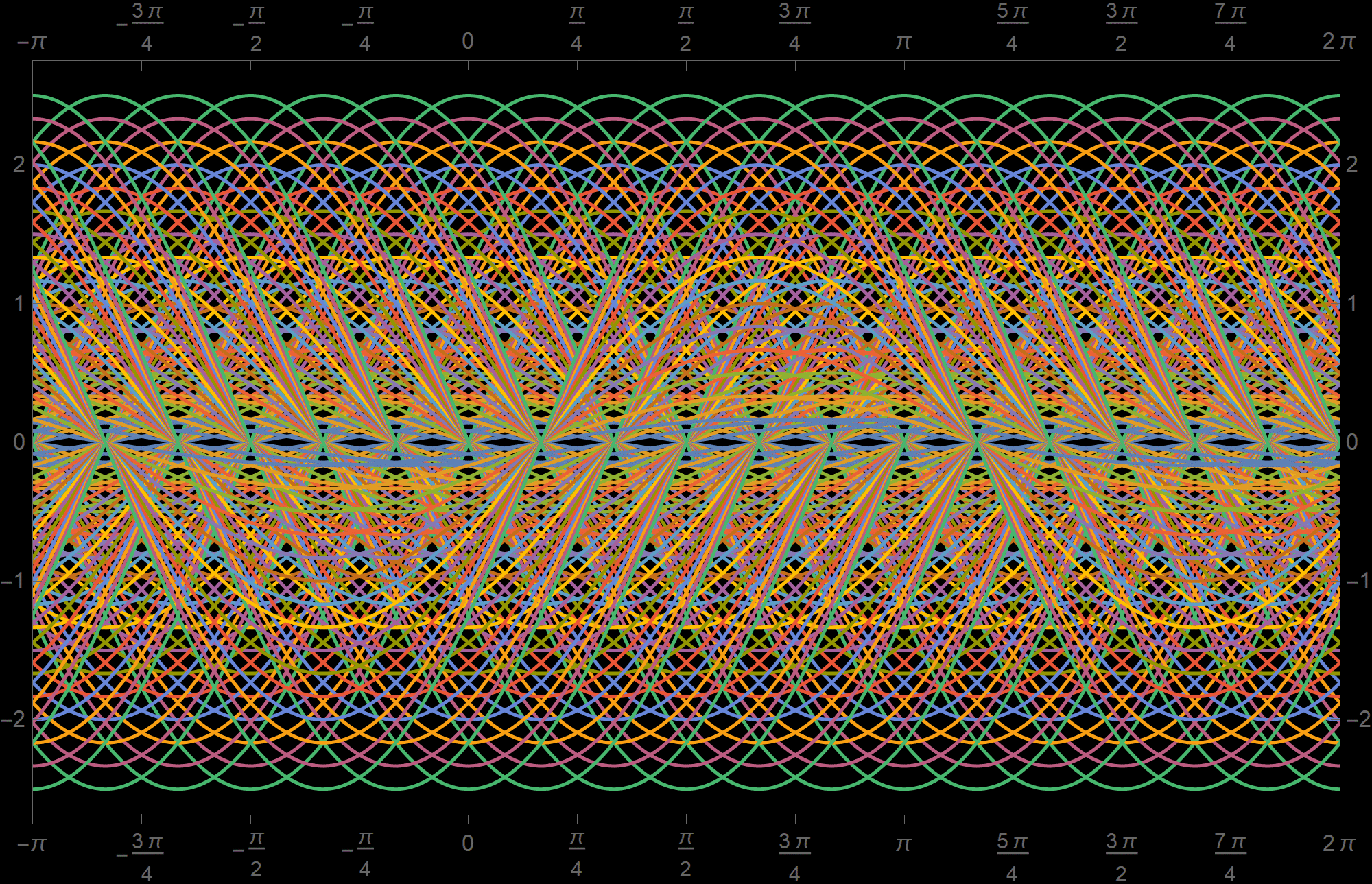
- The above pictures do not directly help us prove that \(\mathcal{S}_1\) is a subspace or determine its dimension. However, they are useful for developing an intuition about what elements of \(\mathcal{S}_1\) look like. We will present a formal proof in the next items. (The proof below is based on knowledge of trigonometry.)
- We will prove the following equality of sets: \[ \mathcal{S}_1 = \operatorname{span}\Bigl\{ \sin(t), \cos(t) \Bigr\}. \]
-
First we prove the inclusion:
\[
\mathcal{S}_1 \subseteq \operatorname{span}\Bigl\{ \sin(t), \cos(t) \Bigr\}.
\]
The inclusion is proved by proving that every element of the set on the left is an element of the set on the right.
Let \(\mathbf{f} \in \mathcal{S}_1\) be arbitrary. By the definition of \(\mathcal{S}_1\) there exist \(a,b \in \mathbb{R}\) such that \[ \mathbf{f}(t) = a \sin(t + b). \] Recall Angle sum and difference identities on Wikipedia, specifically \[ \sin(x+y) = \sin(x) \cos(y) + \cos(x) \sin(y). \] Using this identity we have \begin{align*} \mathbf{f}(t) & = a \sin(t + b) \\ & = a \bigl( \sin(t) \cos(b) + \cos(t) \sin(b) \bigr) \\ & = \bigl(\underbrace{a \cos(b)}_{\alpha} \bigr) \sin(t) + \bigl(\underbrace{a \sin(b)}_{\beta} \bigr) \cos(t) \end{align*}
Setting \(\alpha = a \cos(b)\) and \(\beta = a \sin(b)\) we get \[ \mathbf{f}(t) = \alpha \sin(t) + \beta \cos(t); \] that is \(\mathbf{f}(t)\) is a linear combination of \(\sin(t)\) and \(\cos(t)\). This proves that \[ \mathbf{f} \in \operatorname{span}\Bigl\{ \sin(t), \cos(t) \Bigr\}. \] Since \(\mathbf{f} \in \mathcal{S}_1\) was arbitrary, this proves the inclusion \[ \mathcal{S}_1 \subseteq \operatorname{span}\Bigl\{ \sin(t), \cos(t) \Bigr\}. \]
-
Next we prove the inclusion: \[ \operatorname{span}\Bigl\{ \sin(t), \cos(t) \Bigr\} \subseteq \mathcal{S}_1. \]
Let \(\mathbf{f}(t)\) be an arbitrary element in \(\operatorname{span}\Bigl\{ \sin(t), \cos(t) \Bigr\}\). Then there exist real numbers \(\alpha\) and \(\beta\) such that \[ \mathbf{f}(t) = \alpha \sin(t) + \beta \cos(t). \] If \(\alpha = 0\) and \(\beta = 0\), then we can take \(a = 0\) and \(b=0\) and we have \[ \mathbf{f}(t) = 0 \sin(t) + 0 \cos(t) = 0 \sin(t + 0). \] Therefore \(\mathbf{f} \in \mathcal{S}_1\) in this case.
Now we assume that \(\alpha \neq 0\) or \(\beta \neq 0\). Then \(\alpha^2 + \beta^2 \gt 0\).
At this point the proof uses the unit circle definition of sine and cosine which states: If \(x\) and \(y\) are real numbers such that \(x^2 + y^2 = 1\), then there exists a real number \(\theta\) such that \[ x = \cos(\theta), \quad y = \sin(\theta). \] See Unit circle definition of sine and cosine on Wikipedia.
We use the preceding definition of sine and cosine with \[ x = \frac{\alpha}{\sqrt{\alpha^2 + \beta^2}}, \quad y = \frac{\beta}{\sqrt{\alpha^2 + \beta^2}}. \] Then, \[ x^2 + y^2 = \left(\frac{\alpha}{\sqrt{\alpha^2 + \beta^2}}\right)^2 + \left(\frac{\beta}{\sqrt{\alpha^2 + \beta^2}}\right)^2 = \frac{\alpha^2}{\alpha^2 + \beta^2} + \frac{\beta^2}{\alpha^2 + \beta^2} = 1. \] Consequently, there exists \(\theta \in \mathbb{R}\) such that \[ \cos(\theta) = \frac{\alpha}{\sqrt{\alpha^2 + \beta^2}}, \quad \sin(\theta) = \frac{\beta}{\sqrt{\alpha^2 + \beta^2}}. \]
Using the preceding paragraph we have \begin{align*} \mathbf{f}(t) & = \alpha \sin(t) + \beta \cos(t) \\ & = \sqrt{\alpha^2 + \beta^2} \left( \frac{\alpha}{\sqrt{\alpha^2 + \beta^2}} \sin(t) + \frac{\beta}{\sqrt{\alpha^2 + \beta^2}} \cos(t) \right) \\ & = \sqrt{\alpha^2 + \beta^2} \Bigl( \cos(\theta) \sin(t) + \sin(\theta) \cos(t) \Bigr) \\ & = \sqrt{\alpha^2 + \beta^2} \ \sin(t+\theta). \end{align*} Setting \(a = \sqrt{\alpha^2 + \beta^2}\) and \(b = \theta\) we proved that \[ \mathbf{f}(t) = a \sin(t + b). \] Thus we proved that \(\mathbf{f} \in \mathcal{S}_1\) and this proves that \[ \operatorname{span}\Bigl\{ \sin(t), \cos(t) \Bigr\} \subseteq \mathcal{S}_1. \]
- In conclusion, we proved two inclusions: \begin{align*} \mathcal{S}_1 & \subseteq \operatorname{span}\Bigl\{ \sin(t), \cos(t) \Bigr\} \\ \operatorname{span}\Bigl\{ \sin(t), \cos(t) \Bigr\} & \subseteq \mathcal{S}_1. \end{align*} Therefore, \[ \mathcal{S}_1 = \operatorname{span}\Bigl\{ \sin(t), \cos(t) \Bigr\}. \] Since each span is a subspace this proves that \(\mathcal{S}_1\) is a subspace.
-
To prove that \(\Bigl\{ \sin(t), \cos(t) \Bigr\}\) is a basis for \(\mathcal{S}_1\), we need to prove that \(\sin(t)\) and \(\cos(t)\) are linearly independent. For that we need to prove the implication: \[ \alpha \sin(t) + \beta \cos(t) = 0 \quad \text{for all} \quad t \in \mathbb{R} \] implies \(\alpha = 0\) and \(\beta = 0\).
To prove the last implication, assume \[ \alpha \sin(t) + \beta \cos(t) = 0 \quad \text{for all} \quad t \in \mathbb{R}. \] Setting \(t= 0\) we get \[ 0 = \alpha \sin(0) + \beta \cos(0) = \alpha \, 0 + \beta \, 1 = \beta, \] proving that \(\beta = 0\). Setting \(t = \pi/2\) we get \[ 0 = \alpha \sin(\pi/2) + \beta \cos(\pi/2) = \alpha \, 1 + \beta \, 0 = \alpha, \] proving that \(\alpha = 0\). Thus we proved that \(\alpha = 0\) and \(\beta = 0\). This proves that \(\sin(t)\) and \(\cos(t)\) are linearly independent. Therefore \(\Bigl\{ \sin(t), \cos(t) \Bigr\}\) is a basis for \(\mathcal{S}_1\), Thus, \[ \dim \mathcal{S}_1 = 2. \]
- I created the above animation and the picture with 180 graphs using the computer algebra system Wolfram Mathematica. Enjoyment of mathematics is considerable enriched with Wolfram Mathematica. I would like to encourage you to get familiar with it. To get started with Mathematica see my Mathematica page. Please watch the videos that are on my Mathematica page. Watching the movies is very helpful to get started with Mathematica efficiently! Mathematica is available in the computer labs in BH 215, CF 312, HH 233, and in the Math Center BH 209/211A.
-
In the proof above that \(\mathcal{S}_1\) is a subspace, I used the unit-circle definitions of sine and cosine. What underlies that argument is the idea of polar coordinates.
Polar coordinates often prove invaluable. For example, when working with complex numbers, Euler's identity provides a natural bridge; see the end of this post.
Over the years, I have noticed that students often approach polar coordinates with a certain degree of overconfidence. This topic warrants careful attention. As is often said in discussions about Large Language Models: Attention is All You Need.
-
First I introduce some less common notation.
- We need a fundamental yet often overlooked function, the Unit Step function, for which I will use the patriotic abbreviation \(\operatorname{us}(x)\) with \(x\in \mathbb{R}\). Its definition is as follows: \[ \operatorname{us}(x) = \begin{cases} 1 & \text{if} \quad x \geq 0, \\ 0 & \text{if} \quad x \lt 0. \end{cases} \] This function effectively highlights the dichotomy between nonnegative and negative real numbers.
- By \(\mathbb{R}_+\) we denote the set of positive real numbers; that is \[ \mathbb{R}_{+} = \bigl\{ x \in \mathbb{R} : x \gt 0 \bigr\}. \] With this set notation, the Unit Step function is the indicator function of the set \(\mathbb{R}_+\cup\{0\} \subset \mathbb{R}\).
- Polar Coordinates Theorem. The equations \begin{align*} x & = r \cos\theta, \\ y & = r \sin\theta, \end{align*} establish a bijection between all \((r,\theta)\in\mathbb{R}^+\times (-\pi,\pi]\) and all \((x,y) \in \mathbb{R}^2 \setminus\{(0,0)\}\). Moreover, for \((r,\theta)\in\mathbb{R}^+\times (-\pi,\pi]\) and \((x,y) \in \mathbb{R}^2 \setminus\{(0,0)\}\), the preceding displayed equations are equivalent to \begin{align*} r & = \sqrt{x^2+y^2}, \\ \theta & = \bigl(2\operatorname{us}(y) - 1\bigr) \arccos\biggl( \frac{x}{\sqrt{x^2+y^2}} \biggr). \end{align*}
-
For the proof of the Polar Coordinates Theorem, let \((x,y) \in \mathbb{R}^2\setminus\{(0,0)\}\) and solve the equations \(x= r \cos\theta \) and \(y = r \sin\theta\) for \(r \gt 0\) and \(\theta\in (-\pi,\pi]\).
-
I. First solve the equations \(x= r \cos\theta \) and \(y = r \sin\theta\) for \(r \gt 0\). We have \begin{align*} 0 \lt x^2 + y^2 & = (r \cos\theta)^2 + (r \sin\theta)^2 \\ & = r^2 \bigl( (\cos\theta)^2 + (\sin\theta)^2 \bigr) \\ & = r^2. \end{align*} Thus, since \(r \gt 0\), \[ r = \sqrt{x^2+y^2}. \]
-
II. With the result from I, the point \(\Bigl(\dfrac{x}{r},\dfrac{y}{r}\Bigr)\) is a point on the unit circle. By the definitions of the trigonometric functions cosine and sine there exists a unique \(\theta \in (-\pi,\pi]\) such that \[ \cos\theta = \frac{x}{r} \quad \text{and} \quad \sin\theta = \frac{y}{r}. \] Let us calculate \(\theta \in (-\pi,\pi]\) in terms of \(x\) and \(y\). Notice that for all \((x,y) \in \mathbb{R}^2\setminus\{(0,0)\}\) we have \[ \frac{x}{\sqrt{x^2+y^2}} \in [-1,1]; \] that is \( \dfrac{x}{\sqrt{x^2+y^2}}\) is in the domain of the inverse trigonometric function \(\arccos:[-1,1] \to [0,\pi]\). This observation is the key for this proof.
-
III. If \(y \geq 0\), then by the definition of the inverse trigonometric function \(\arccos:[-1,1] \to [0,\pi]\) we have \[ \theta = \arccos\biggl( \frac{x}{\sqrt{x^2+y^2}} \biggr) \in [0,\pi]. \] Let us prove that this \(\theta \in [0,\pi]\) is the solution that we seek. With this \(\theta \in [0,\pi]\) we have \(\cos\theta = \frac{x}{r}\). Furthermore, since \((\cos\theta)^2 + (\sin\theta)^2=1\), we have \[ (\sin\theta)^2 = 1 - \frac{x^2}{x^2+y^2} = \frac{y^2}{x^2+y^2}. \] As both \(\sin\theta \geq 0\) and \(y \geq 0\), we deduce \(\sin\theta = \frac{y}{r}\), and thus \[ \cos\theta = \frac{x}{r} \quad \text{and} \quad \sin\theta = \frac{y}{r} \geq 0, \] the desired equalities hold.
-
IV. If \(y \lt 0\), then, with the above defined \(\theta\), we have \(\theta \in (0,\pi)\) and, by the calculations in III, \[ \cos\theta = \frac{x}{r} \quad \text{and} \quad \sin\theta = \frac{|y|}{r} \gt 0. \] Therefore, with \(-\theta \in (-\pi,0)\) we have \[ \cos(-\theta) = \cos\theta = \frac{x}{r} \quad \text{and} \quad \sin(-\theta) = -\sin\theta = -\frac{|y|}{r} = \frac{y}{r} \lt 0, \] the desired equalities again hold.
-
V. Since \[ 2\operatorname{us}(y) - 1 = \begin{cases} \phantom{-}1 & \text{if} \quad y \geq 0, \\ -1 & \text{if} \quad y \lt 0, \end{cases} \] we can unify the results from III and IV and set \[ \theta = \bigl(2\operatorname{us}(y) - 1\bigr) \arccos\biggl( \frac{x}{\sqrt{x^2+y^2}} \biggr). \] If \(y \geq 0\), then, by III, we have \(x= r \cos\theta \) and \(y = r \sin\theta\). If \(y \lt 0\), then, by IV, we have \(x= r \cos\theta \) and \(y = r \sin\theta\). In conclusion with \(\theta\) given in the last displayed equality we have both desired equalties regardless of the sign of \(y\).
-
-
This completes the proof of the Polar Coordinates Theorem.
-
Since I spent all this space on the details of polar coordinates, let me recall that in the context of complex numbers there is standard terminology for all four real numbers \(x\), \(y\), \(r\), \(\theta\) introduced in the Polar Coordinates Theorem.
\(z= x + \mathrm{i}\mkern 2mu y = r e^{\mathrm{i}\mkern 2mu\theta}\) Terminology Notation \(x\) the real part of \(z\) \(\operatorname{Re}(z)\) \(y\) the imaginary part of \(z\) \(\operatorname{Im}(z)\) \(r\) the modulus of \(z\) \(|z|\) \(\theta\) the principal argument of \(z\) \(\operatorname{Arg}(z)\) -
The website Argument (complex analysis) - Wikipedia distinguishes the principal value of the argument, denoted by \(\operatorname{Arg}(z)\), and the multivalued function \(\arg(z)\). I have seen \(\arg(z)\) used as the notation for the principal value.
I am proud to promote the simple formula for the principal value of the argument: \(\theta = \operatorname{Arg}(z) \in (-\pi,\pi]\) using the Unit Step function: For \(\mathbb{C}\setminus\{0\}\) we have \[ \theta = \operatorname{Arg}(z) = \Bigl(2\operatorname{us}\bigl(\operatorname{Im}(z)\bigr) - 1\Bigr) \arccos\biggl( \frac{\operatorname{Re}(z)}{|z|} \biggr). \]
For \((x,y) \in \mathbb{R}^2\setminus\{(0,0)\}\), compare this simple formula to the function \(\operatorname{atan\mkern-3mu 2}\) at Computing from the real and imaginary part - Wikipedia \[ \operatorname{Arg}(x + iy) = \operatorname{atan\mkern-3mu 2}(y,\, x) = \begin{cases} \arctan\left(\frac y x\right) &\text{if } x \gt 0, \\[5mu] \arctan\left(\frac y x\right) + \pi &\text{if } x \lt 0 \text{ and } y \ge 0, \\[5mu] \arctan\left(\frac y x\right) - \pi &\text{if } x \lt 0 \text{ and } y \lt 0, \\[5mu] +\frac{\pi}{2} &\text{if } x = 0 \text{ and } y \gt 0, \\[5mu] -\frac{\pi}{2} &\text{if } x = 0 \text{ and } y \lt 0. \end{cases} \] I am not sure why they use \(\arctan\) when \(\arccos\) is much simpler: \[ \operatorname{atan\mkern-3mu 2}(y,\, x) = \bigl(2\operatorname{us}(y) - 1\bigr) \arccos\biggl( \frac{x}{\sqrt{x^2+y^2}} \biggr). \] My only explanation is that they are afraid of \(\sqrt{x^2+y^2}\).
- I disclose that I borrowed the code for the long cases formula for \(\operatorname{atan\mkern-3mu 2}\) from the Wikipedia site by clicking the Edit link next to the title. It is all in LaTeX. The table with terminology was generated by ChatGPT. My HTML skills are not that good.
- I updated my notes on Vector Spaces (updated). I added the important and scary example of the zero vector space. In class you requested more basic properties, so I added one more, the uniqueness of the zero vector. The same notes with cropped pages.
-
In class I mentioned Terence Tao's Quote on the Humbling Nature of Mathematics. As far as I could find out he mentioned it in two YouTube podcases Lex Fridman Podcast (Episode 472, June 2024) and Dr Brian Keating. Below is how Gemini summarized Tao's thinking.
In a recent appearance on podcasts world-renowned mathematician Terence Tao discussed why the rigorous nature of mathematical proof acts as a powerful check on one's ego.
Unlike other fields where reputation can carry an argument, Tao explained that mathematics is objective—either a proof works, or it doesn't. Here is the key insight from that conversation:
"One thing that helps ground mathematicians a little bit is that... as a pure mathematician, your main task is you have these problems you want to solve, and you want to prove theorems that solve these problems. And your proof has to be correct, and every step has to be validated. And it doesn't matter how famous you are or how much of a reputation you have, you can't just say 'I've proven something, trust me.' You have to supply the details. And if you don't have the proof, you don't have the proof. So I think this naturally provides some check on just how high your ego can go... despite the awards. Because, you know, I mean there are countless problems that I would love to solve—you know the twin prime conjecture we talked about, but hundreds of problems that I would love to solve—and I just know I don't know how to solve. And so I know more problems I can't solve than the problems I have solved. So I think that... so that keeps you somewhat honest."
He further emphasized the clarity of failure in the field, noting, "It’s a specific feature of math that you can be wrong very explicitly."
Tao's thinking about LLMs:
"So we have to reinvent the way we teach. So, um, one thing that will become more important is students will need to have much more training in how to validate information that they see. I think as long as you pair these AIs with good verification, and you only use the AIs to the extent that you can verify the outputs—and no further—then they can be a great tool. I see them more as complimenting human scientists and mathematicians. Because there are so few human scientists in the world and we only have so much time to work on research, we tend to focus on sort of high value, high priority, isolated problems. But in mathematics and the sciences, there is a long tail of lots and lots of less well-known problems which should require some attention. They're not the most difficult or important, but it'll be good to have someone or something look at them. And so I think AI actually, their best use case is not to target them on the most high-profile problems but actually on the millions of medium difficulty problems. And you know, they may fail and they may only solve 10% of these million problems, but that's 100,000 problems solved. So scale is the big advantage. You know, you cannot scale a graduate student this way."
The entire podcast:
- I updated my notes on Vector Spaces. I corrected the errors that you pointed out today and added some more content that I presented in class. The same notes with cropped pages.
-
The reading from the textbook:
- Section 1A in the textbook: Review of complex numbers, the concept of a list (I prefer to call lists tuples), the space $\mathbb{F}^n$ (Notice that in this book the author uses the old-fashioned bold face capitals to denote the scalar fields. I prefer to use, so called blackboldbold font, which seems to be more common nowdays.)
- Section 1B in the textbook: Definition of a vector space and exercises.
- If you find an exercise that you cannot solve, please report them in Discussions on Canvas.
- My notes on Complex Numbers. There are 11 exercises at the end of my notes. Almost entirely the content of my notes is mentioned in the Common Core State Standards for Mathematics. Some of the exercises are very similar to the exercises mentioned in the Common Core State Standards for Mathematics.
- My notes on Mathematical Logic. The same notes with cropped pages.
- My notes on Vector Spaces.
- Professor Sheldon Axler, the author of Linear Algebra Done Right has made PDF file of the fourth edition of this popular linear algebra book available free of charge. We are taking advantage of this generous gesture and we are using this book this quarter.
- The information sheet
- Some relevant Wikipedia links:
-
Before briefly reflecting on the history of Linear Algebra, I want to celebrate the history of mathematics with a short paragraph:
Throughout history, human civilizations have developed and shared mathematical knowledge. Successive civilizations have recognized and admired the contributions of those who came before. Earlier discoveries have provided both a foundation and an inspiration for further advances, giving mathematics the spirit of a collective endeavor of humanity across the past, the present, and the future.
-
What is the oldest linear algebra problem?
-
Clay tablet VAT 8389 from the Old Babylonian period, from 2000 to 1600 BC, contains what is believed to be the earliest word problem that can be interpreted as a system of linear equations:
A translation of this word problem into a system of linear equations is as follows: \begin{alignat*}{4} &x_1 & &\ + &x_2 & = 1800 \\ \tfrac{2}{3} &x_1 & &- \tfrac{1}{2} &x_2 & = \phantom{1}500. \end{alignat*} -
Problem 40 of the Rhind papyrus which is dated to 1550 BC is:
Denote by $x_1$ the smallest number and by $x_2$ the common difference. After simplification the above problem translates into the following system of linear equations: \begin{alignat*}{5} 5 &x_1 & & + 10 &x_2 & = 100 \\ \tfrac{11}{7} &x_1 & & - \phantom{1}\tfrac{2}{7} &x_2 & = \phantom{10}0. \end{alignat*} -
Most importantly for us, the oldest known treatment of systems of linear equations from antiquity which resembles the methods that we will use in this class is in Chapter 8 of the Chinese textbook Nine Chapters of the Mathematical Art which is at least 1800 years old.
-
Clay tablet VAT 8389 from the Old Babylonian period, from 2000 to 1600 BC, contains what is believed to be the earliest word problem that can be interpreted as a system of linear equations: