- The notebook Super_glued_ends_solution_v12.nb contains a Mathematica implementation of finding a solution of the vibrating string equation with a Robin boundary condition. A pdf printout of this notebook is Super_glued_ends_solution_v12.pdf. You can download the Mathematica notebook here Super_glued_ends_solution_v12.nb
-
Let $L \gt 0$, \(c\gt 0\), and $h \in \mathbb{R}.$ Let $f:[0,L]\to\mathbb{R}$ and $g:[0,L]\to\mathbb{R}$ be continuous functions whose derivatives are piecewise continuous. We consider the vibrating string equation with a Robin boundary condition at $0$ and the Diriclet boundary condition at $L$:
\begin{alignat*}{2}
&\text{PDE:} \qquad & & \frac{\partial u^2}{\partial t^2}(x,t) = c^2 \frac{\partial u^2}{\partial x^2}(x,t)
\quad \text{where} \quad x \in [0,\pi] \quad \text{and} \quad t \in [0,+\infty) \\
&\text{BCs:} \qquad & & u(0,t) - h \frac{\partial u}{\partial x}(0,t) = 0 \quad \text{and} \quad u(L,t) = 0
\quad \text{for all} \quad t \in [0,+\infty), \\
&\text{ICs:} \qquad & & u(x,0) = f(x) \quad \text{and} \quad \frac{\partial u}{\partial t}(x,0) = g(x)
\quad \text{for all} \quad x \in [0,L].
\end{alignat*}
On Thursday and Friday we analyzed "natural modes of vibration" of this string for all possible cases of $L \gt 0$ and $h \in \mathbb{R}.$ There are three distinct cases:
-
Case 1. $-L \lt h \lt 0$ In this case, there is one negative eigenvalue and countably many positive eigenvalues. For a general choice of the initial shape $f(x)$ and the initial velocity $g(x)$ the string will break in this case. See the the animation below.
Place the cursor over the image to start vibrations.

However, if we set the initial velocity $g(x)= 0$ and we make a special choice of the initial shape $f(x)$ that is orthogonal to the eigenfunction corresponding to the negative eigenvalue than the string does not break. See the animation below.
Place the cursor over the image to start vibrations.
-
Case 2. $h = -L$ In this case, $0$ is an eigenvalue and there are countably many positive eigenvalues. For a general choice of the initial shape $f(x)$ and no initial velocity, that is $g(x) = 0,$ the string will not break. This is illustrated in the animation below with $L = \pi$ and $h=-\pi$.
Place the cursor over the image to start vibrations.
For a general choice of the initial velocity $g(x)$ the string breaks. We did not illustrate this case.
-
Case 3. $h \geq 0$ or $h \leq -L$ In this case, there are no negative eigenvalues, $0$ is not an eigenvalue and there are countably many positive eigenvalues. See the animation below with $L =\pi$ and $h=-4$.
Place the cursor over the image to start vibrations.
In the animation below we used $L =\pi$ and $h=1$.
Place the cursor over the image to start vibrations.
-
- The relevant part from the textbook is Section 5.8.
-
The book talks about various kinds of boundary conditions for the vibrating string equation in Section 4.2 and Section 4.3. Today I presented my way to explaining how the boundary conditions of the "third kind" or Robin boundary conditions arise naturally.
I wrote the notes about my approach the boundary conditions of the "third kind" or Robin boundary conditions. These notes present a method of solving boundary eigenvalue problems with the boundary conditions of the "third kind" or Robin boundary conditions (the boundary conditions discussed today). The relevant part from the textbook is Section 5.8.
-
Today we introduced the boundary conditions of the "third kind" or Robin boundary conditions for the vibrating string equation. In my interpretation, these boundary conditions describe a string with a rigid end (sometimes I say, an end soaked in super-glue) as in the animation below. In the animation below, the left end of the string soaked in super-glue is of length $h=1$. The resulting boundary condition at the endpoint $0$ is
\[
u(0,t) - 1 \frac{\partial u}{\partial x}(0,t) = 0.
\]
This is a Robin boundary condition. The general Robin boundary condition at the endpoint \(0\) is
\[
u(0,t) - h \frac{\partial u}{\partial x}(0,t) = 0.
\]
The general Robin boundary condition at the endpoint \(0\) arises when a part of the string of length \(h \gt 0\) is soaked in super-glue.
Place the cursor over the image to start vibrations.
Notice that the red part of the string is rigid, while the orange part is governed by the vibrating string equation.
- The goal of the notes is to explain how to solve the vibrating string equation with a Robin boundary condition. That is, how to obtain the above presented animation. The notes complement Section 5.8 of the book.
-
On Friday, we used Fourier's Method of Separation of Variables to find two sequences of solutions oto the Vibrating String Partial Differential Equation \[ \frac{\partial^2u}{\partial t^2}(x,t) = c^2 \frac{\partial^2 u}{\partial x^2}(x,t), \quad \text{where} \quad x \in [0,L], \ \ t \geq 0, \] subject to Dirichlet Boundary Conditions at the endpoints \(0\) and \(L\): \[ u(0,t) = 0 \quad \text{and} \quad u(L,t) = 0, \quad \text{for all} \quad t \geq 0. \]
- Two sequences of solutions are \[ \cos\biggl(\frac{k\pi c}{L} t \biggr)\sin\biggl(\frac{k\pi}{L} x \biggr) \quad \text{and} \quad \sin\biggl(\frac{k\pi c}{L} t \biggr)\sin\biggl(\frac{k\pi}{L} x \biggr), \quad \text{where} \quad k \in \mathbb{N}. \] I want to illustrate these solutions by animations of their vibrations. It is important to notice that, for a fixed \(k\), looking at the vibrations of these solutions do not differ at all. The reason for this is that the sine function in time \(t\) is a shift of the cosine function, the shift by \( \dfrac{L}{2k c} \) in this case. Thus, I present only the solution with the cosine time part. If you want to think of the vibrations of a solution with the sine time part, then instead of starting at time \(t = 0\), you think of time starting at \(t=L/(2kc)\).
- Below I present the solutions for \(k \in \{1,2,3,4,5,6\}\) with \(L=\pi\) and \(c=1\). These solutions are called the natural modes of vibration of a string with fixed endpoints. For each picture hover the cursor over the image to start vibrations.
- It is really remarkable that we can find the exact solution of the vibrating string equation with the initial condition of the specific trigonometric form. For this we need to review some beautiful trigonometric identities.
- Since we work with trigonometric functions a lot, it is helpful to review beautiful world of trigonometric identities. The Wikipedia page List_of_trigonometric_identities is a good place for such a review.
-
One particular kind of trigonometric identities are Power reduction formulas. Below I list several such formulas which involve multiple-angle sine functions in \(x\); exactly the kind that we encountered as solutions of the vibrating string equation.
In the context of Fourier series, the trigonometric identities listed below are important since they are in fact finite Fourier series (here \(L=\pi\)) for the functions appearing on the left-hand side of the identities.
\begin{align*} (\sin x)^3 & = \frac{3}{4}\sin(x) - \frac{1}{4} \sin(3 x)\\ (\sin x)^5 & = \frac{5}{8}\sin (x) - \frac{5}{16} \sin (3 x)+\frac{1}{16} \sin (5 x)\\ \bigl(\sin x\bigr)^{7} & = \frac{35}{64}\sin(x) - \frac{21}{64}\sin(3x) + \frac{7}{64}\sin(5x) - \frac{1}{64} \sin(7x), \\[6pt] (\sin x)^9 &= \frac{63}{128} \sin x - \frac{21}{64} \sin(3x) + \frac{9}{64} \sin(5x) - \frac{9}{256} \sin(7x) + \frac{1}{256} \sin(9x). \end{align*}
\begin{align*} (\sin x)(\cos x) & = \frac{1}{2} \sin (2 x) \\ (\sin x)(\cos x)^2 & = \frac{1}{4} \sin (x) + \frac{1}{4} \sin (3 x) \\ (\sin x)(\cos x)^3 & = \frac{1}{4} \sin (2 x) + \frac{1}{8} \sin (4 x) \\ (\sin x)(\cos x)^4 & = \frac{1}{8} \sin (x) + \frac{3}{16} \sin (3 x) + \frac{1}{16} \sin (5 x) \\ (\sin x)(\cos x)^5 & = \frac{5}{32} \sin (2x) + \frac{1}{8} \sin (4 x) + \frac{1}{32} \sin (6 x) \\ (\sin x)^3 & = \frac{3}{4} \sin (x) - \frac{1}{4} \sin (3 x) \\ (\sin x)^3(\cos x) & = \frac{1}{4} \sin (2 x) - \frac{1}{8} \sin (4 x) \\ (\sin x)^3 (\cos x)^2 & = \frac{1}{8} \sin (x) + \frac{1}{16} \sin (3 x) - \frac{1}{16} \sin (5 x) \\ (\sin x)^3(\cos x)^3 & = \frac{3}{32} \sin (2 x) - \frac{1}{32} \sin (6 x) \\ (\sin x)^3(\cos x)^4 & = \frac{3}{64} \sin (x) + \frac{3}{64} \sin (3 x) - \frac{1}{64} \sin (5 x) - \frac{1}{64} \sin (7 x) \\ (\sin x)^3(\cos x)^5 & = \frac{3}{64} \sin (2 x) + \frac{1}{64} \sin (4 x) - \frac{1}{64} \sin (6 x) - \frac{1}{128} \sin (8 x) \\ \end{align*}
In the context of this class, each of the above formulas gives a finite Fourier series for the function on the left-hand side of the equality sign.
Also, the above formulas, though not immediately apparent, contain numerous integrals in a disguised form. For example, \[ \int_{-\pi} ^{\pi} (\sin x)^3(\cos x)^4 \sin (3 x) dx = \frac{3 \pi}{64}, \] but also \[ \int_{-\pi} ^{\pi} (\sin x)^3(\cos x)^4 \sin (4 x) dx = 0. \] Do you see why?
- Next, we will use the above trigonometric identities to obtain a formula for the solution of a particular vibrating string equation with Dirichelt boundary conditions and given initial displacement and initial velocity being \(0\): \[ \frac{\partial^2u}{\partial t^2}(x,t) = \frac{\partial^2 u}{\partial x^2}(x,t), \quad \text{where} \quad x \in [0,\pi], \ \ t \geq 0, \] subject to Dirichlet Boundary Conditions at the endpoints \(0\) and \(\pi\): \[ u(0,t) = 0 \quad \text{and} \quad u(\pi,t) = 0, \quad \text{for all} \quad t \geq 0, \] and the following initial conditions: for all \(x \in [0,\pi]\) \begin{align*} u(x,0) & = (\sin x)^3 +(\sin x) (\cos x)^3 \\ \frac{\partial u}{\partial t}(x,0) &= 0. \end{align*}
- Since \[ (\sin x)^3 = \frac{3}{4}\sin(x) - \frac{1}{4} \sin(3 x) \] and \[ (\sin x)(\cos x)^3 = \frac{1}{4} \sin (2 x) + \frac{1}{8} \sin (4 x), \] we have that \begin{align*} u(x,0) & = (\sin x)^3 +(\sin x) (\cos x)^3 \\ & = \frac{3}{4}\sin(x) + \frac{1}{4} \sin (2 x) - \frac{1}{4} \sin(3 x) + \frac{1}{8} \sin (4 x). \end{align*} Therefore, the exact solution of the given vibrating string equation with the Dirichlet boundary and the given initial displacement and \(0\) initial velocity is given by \[ u(x,t) = \frac{3}{4}(\cos t) (\sin x) + \frac{1}{4} \cos(2 t) \sin (2 x) - \frac{1}{4} \cos(3 t) \sin(3 x) + \frac{1}{8} \cos(4 t) \sin (4 x). \] Below is an animation of the solution.
-
If the initial conditions are functions for which we do not have explicit formulas in terms of the multiple-angle sine functions, then we need to calculate the Fourier coefficients of the functions given as the initial conditions. That requires use of technology, and often the coefficients need to be calculated approximately.
-
For example, consider the following initial conditions: \begin{align*} u(x,0) & = \frac{1}{6} (\pi -x) x^2 \\[5pt] \frac{\partial u}{\partial t}(x,0) &= 0. \end{align*}
Since the initial velocity is \(0\), the solution has the form \[ u(x,t) = \sum_{k=1}^\infty c_k \cos(k \pi t) \sin(k \pi x). \] We choose the coefficients \(c_k\) such that \[ u(x,0) = \frac{1}{6} (\pi -x) x^2 = \sum_{k=1}^\infty c_k \sin(k \pi x). \] The orthogonality of the multiple-angle sine functions we calculate \[ c_k = \frac{1}{3 \pi} \int_{0}^\pi (\pi -x) x^2 \sin(k \pi x) \operatorname{d}\mkern-2mu x \] Wolfram Mathematica calculates the above integral and gives: \[ c_k = -\frac{2 \left(2 (-1)^k+1\right)}{3 k^3} \]
Thus, the solution given as an infinite sum is \[ u(x,t) = - \frac{2}{3} \sum_{k=1}^\infty \frac{2 (-1)^k+1}{k^3} \mkern 2mu \cos(k \pi t) \sin(k \pi x). \]
Choosing the partial sum with \(50\) terms of the above infinite series we get the following animation of the solution: -
Consider more a complicated function for the initial displacement. For example, consider the following initial conditions: \begin{align*} u(x,0) & = \frac{4}{\pi ^2} x (\pi -x) e^{-5 (x-1)^2} \\[5pt] \frac{\partial u}{\partial t}(x,0) &= 0. \end{align*}
Since the initial velocity is \(0\), the solution has the form \[ u(x,t) = \sum_{k=1}^\infty c_k \cos(k \pi t) \sin(k \pi x). \] We choose the coefficients \(c_k\) such that \[ u(x,0) = \frac{1}{6} (\pi -x) x^2 = \sum_{k=1}^\infty c_k \sin(k \pi x). \] The orthogonality of the multiple-angle sine functions we calculate \[ c_k = \frac{2}{\pi} \int_{0}^\pi \frac{4}{\pi ^2} x (\pi -x) e^{-5 (x-1)^2} \sin(k \pi x) \operatorname{d}\mkern-2mu x \] Wolfram Mathematica cannot find the exact formulas for these coefficients. Therefore, I calculated numerical approximations for the first \(50\) coefficients and obtained an approximation for the solution. Below is the resulting animaltion:
-
The above animations are created in the Mathematica notebook linked below
- Natural_modes_of_vibration.nb Here is the pdf printout of the same notebook.
- This is in Sections 4.4 in the book.
- I created this small Mathematica notebook in which I explain how to create animations and export them as common animated files. Here is the pdf printout of the same notebook.
-
Below is an animated gif that I produced
 Below is an animated png that I produced
 There is not much difference in quality. For more complicated pictures I think that png format is better.
- Unfortunately I did not find a simple way to include animated files in pdf documents. As you can see from my website, it is easy to include animated gifs and animated pngs in html files. These files show nicely in browsers.
the first harmonic or fundamental
the second harmonic
the third harmonic
the fourth harmonic
the fifth harmonic
the sixth harmonic
Place the cursor over the image to start vibrations.
Place the cursor over the image to start vibrations.
Place the cursor over the image to start vibrations.
- Yesterday I posted several theorems about term-by-term differentiation and integration of Fourier series. These are Sections 3.4 and 3.5 in the book. Since we don't have much time left in the quarter, we will skip this topic and move on to the vibrating string equation.
-
Today we derived the partial differential equation which models vibrations of a string. This is Section 4.2 in the book. The simplest form of this equation is \[ \frac{\partial^2u}{\partial t^2}(x,t) = c^2 \frac{\partial^2 u}{\partial x^2}(x,t) \quad \text{where} \quad x \in [0,L], \ \ t \geq 0. \] This equation is called vibrating string equation, or one-dimensional wave equation. In this equation, we think of the string in the equilibrium position is scratched along the \(x\)-axis from \(0\) to \(L\). Then, as string vibrates, the small value \(u(x,t)\) represents the displacement of the string at the position \(x \in [0,L]\) at time \(t\). The positive values of \(u(x,t)\) represent the displacement above the \(x\)-axis and the negative values of \(u(x,t)\) represent the displacement below the \(x\)-axis.
Natural boundary conditions are that the string is fixed at its endpoints \(0\) and \(L\): \[ u(0,t) = 0 \quad \text{and} \quad u(L,t) = 0 \quad \text{for all} \quad t \geq 0. \]
-
Set \(L = \pi\) and \(c=1\) in the vibrating string equation and consider the vibrating string equation \[ \frac{\partial^2 u}{\partial t^2}(x,t) = \frac{\partial^2 u}{\partial x^2}(x,t) \quad \text{where} \quad x \in [0,\pi], \ \ t \geq 0, \] subject to the boundary conditions \[ u(0,t) = 0 \quad \text{and} \quad u(\pi,t) = 0 \quad \text{for all} \quad t \geq 0. \]
-
One solution of this equation is \[ u(x,t) = (\cos t) (\sin x). \] To verify this claim calculate \begin{align*} \frac{\partial^2}{\partial t^2}\bigl( (\cos t) (\sin x) \bigr) & = - (\cos t) (\sin x) \\ \frac{\partial^2}{\partial x^2}\bigl( (\cos t) (\sin x) \bigr) & = - (\cos t) (\sin x), \end{align*} and \[ (\cos t) (\sin 0) = (\cos t) (\sin \pi ) = 0. \]
Animating the function \[ (\cos t) (\sin x) \] in time we obtain the animation below, which really resembles vibrations of a string. In the animation below we let \(t\) run from \(0\) to \(2\pi\). Since \(\cos t\) is periodic, the animation appears to continue infinitely.
-
Another solution of the same vibrating string equation is \[ u(x,t) = \bigl(\cos (2t) \bigr) \bigl(\sin(2x) \bigr). \] To verify this claim calculate \begin{align*} \frac{\partial^2}{\partial t^2}\Bigl( \bigl(\cos (2t) \bigr) \bigl(\sin(2x) \bigr) \Bigr) & = - 4 \bigl(\cos (2t) \bigr) \bigl(\sin(2x) \bigr) \\ \frac{\partial^2}{\partial x^2} \Bigl( \bigl(\cos (2t) \bigr) \bigl(\sin(2x) \bigr) \Bigr) &= - 4 \bigl(\cos (2t) \bigr) \bigl(\sin(2x) \bigr), \end{align*} and \[ \bigl(\cos (2t) \bigr) \bigl(\sin(2\times 0) \bigr) = \bigl(\cos (2t) \bigr) \bigl(\sin(2 \pi) \bigr) = 0. \]
Animating the function \[ \bigl(\cos (2t) \bigr) \bigl(\sin(2x) \bigr) \] in time we obtain the animation below, which really resembles vibrations of a string. In the animation below we let \(t\) run from \(0\) to \(2\pi\). Since \(\cos t\) is periodic, the animation appears to continue infinitely.
-
-
We first prove a Differentiation Theorem for Fourier Series.
Differentiation term-by-term Theorem. Let $L \gt 0$ and let $f:[-L,L] \to \mathbb R$ be a function. Assume that
- $f$ is continuous on the closed interval $[-L,L],$
- $f$ is piecewise smooth function on $[-L,L],$
- $f'$ is piecewise smooth function on $[-L,L],$
Proof. Since $f'$ is piecewise smooth its Fourier series converges pointwise to the Fourier periodic extension of $f'.$ Denote the coefficients of this Fourier series by $\alpha_0,$ $\alpha_k$ and $\beta_k.$ Let us calculate $\alpha_0.$ Since $f$ is continuous and $f'$ is piecewise continuous the Fundamental Theorem of Calculus applies and it yields \[ \alpha_0 = \frac{1}{2L} \int_{-L}^L f'(x) dx = \frac{1}{2L} \bigl( f(L) - f(-L) \bigr). \] Let us calculate $A_k$. Since $f(x)\cos\bigl(k\pi x/L\bigr)$ is continuous and $f'$ is piecewise continuous the Integration by Parts Theorem applies and it yields \begin{align*} \alpha_k & = \frac{1}{L} \int_{-L}^L f'(x) \cos\left(\frac{k \pi}{L} x\right) dx \\ & = \frac{1}{L} \left( f(L) \cos\bigl(k\pi\bigr) - f(-L) \cos\bigl(-k\pi\bigr) + \frac{k \pi}{L} \int_{-L}^L f(x) \sin\left(\frac{k \pi}{L} x\right) dx \right) \\ & = \frac{1}{L} \left( (-1)^k \bigl( f(L) - f(-L) \bigr) + \frac{k \pi}{L} \int_{-L}^L f(x) \sin\left(\frac{k \pi}{L} x\right) dx \right) \\ & = \frac{1}{L} \Bigl( (-1)^k \bigl( f(L) - f(-L) \bigr) + k \pi \, b_k \Bigr) \\ \end{align*} Let us calculate $B_k$. Since $f(x)\sin\bigl(k\pi x/L\bigr)$ is continuous and $f'$ is piecewise continuous the Integration by Parts Theorem applies and it yields \begin{align*} \beta_k & = \frac{1}{L} \int_{-L}^L f'(x) \sin\left(\frac{k \pi}{L} x\right) dx \\ & = \frac{1}{L} \left( f(L) \sin\bigl(k\pi\bigr) - f(-L) \sin\bigl(-k\pi\bigr) - \frac{k \pi}{L} \int_{-L}^L f(x) \cos\left(\frac{k \pi}{L} x\right) dx \right) \\ & = \frac{1}{L} \left( - k \pi \, a_k \right) \end{align*} -
The book proves the following Differentiation Theorem for Fourier sine series.
- $f$ is continuous on the closed interval $[0,L],$
- $f$ is piecewise smooth function on $[0,L],$
- $f'$ is piecewise smooth function on $[0,L].$
-
Here we prove Integration term-by-term Theorem for Fourier series.
Integration term-by-term Theorem. Let $L \gt 0$ and let $f:[-L,L] \to \mathbb R$ be a function. Assume that
- $f$ is piecewise smooth function on $[-L,L],$
- $\displaystyle a_0 = \frac{1}{2L} \int_{-L}^{L} f(\xi) d\xi = 0,$
- $\displaystyle F(x) = \int_{0}^{x} f(\xi) d\xi.$
Proof of Integration term-by-term Theorem. Since we assume \[ 0 = \int_{-L}^{L} f(\xi) d\xi = -\int_{0}^{-L} f(\xi) d\xi + \int_{0}^{L} f(\xi) d\xi = -F(-L) + F(L), \] the periodic extension $\widetilde F$ of $F$ is continuous and piecewise smooth. Therefore its Fourier series converges uniformly to $\widetilde F$. Let us now calculate the Fourier series of $F.$ Denote the coefficients of this Fourier series by $A_0,$ $A_k$ and $B_k.$ It is tricky to calculate $A_0,$ so we postpone it for the end of the proof. However, in each practical situation this will be the easiest one to calculate since it is the average value of $F$ on $[-L,L].$ The difficulty here arises from the fact that the average value of $F$ on $[-L,L]$ cannot be expressed directly in terms of $f.$
Let us calculate $A_k$. Since $F(x)\cos\bigl(k\pi x/L\bigr)$ is continuous and $f(x)$ is piecewise continuous the Integration by Parts Theorem applies and it yields \begin{align*} A_k & = \frac{1}{L} \int_{-L}^L F(\xi) \cos\left(\frac{k \pi}{L} \xi \right) dx \\ \fbox{Integration by Parts} & = \frac{1}{L} \left( \frac{L}{k\pi} F(L) \sin\bigl(k\pi\bigr) - \frac{L}{k\pi} F(-L) \sin\bigl(-k\pi\bigr) - \frac{L}{k\pi} \int_{-L}^L f(\xi) \sin\left(\frac{k \pi}{L} \xi\right) d\xi \right) \\ \fbox{since \(\ \sin\bigl(k\pi\bigr) =0\)} & = - \frac{L}{k \pi} b_k \end{align*} Let us calculate $B_k$. Since $F(x)\sin\bigl(k\pi x/L\bigr)$ is continuous and $f$ is piecewise smooth the Integration by Parts Theorem applies and it yields \begin{align*} B_k & = \frac{1}{L} \int_{-L}^L F(\xi) \sin\left(\frac{k \pi}{L} \xi \right) d\xi \\ \fbox{Integration by Parts} & = \frac{1}{L} \left( - \frac{L}{k\pi} F(L) \cos\bigl(k\pi\bigr) + \frac{L}{k\pi} F(-L) \cos\bigl(k\pi\bigr) + \frac{L}{k\pi} \int_{-L}^L f(\xi) \cos\left(\frac{k \pi}{L} \xi\right) d\xi \right) \\ \fbox{since \(\ F(L) = F(-L)\)} & = \frac{L}{k \pi} a_k \end{align*} Hence, for all $x\in \mathbb{R}$ we have \[ {\widetilde F}(x) = A_0 - \frac{L}{\pi} \sum_{k=1}^{\infty} \frac{b_k}{k} \cos\left(\frac{k\pi}{L} x \right) + \frac{L}{\pi} \sum_{k=1}^{\infty} \frac{a_k}{k} \sin\left(\frac{k\pi}{L} x \right). \] In particular the preceding equality holds for $x=0.$ Since $F(0) = 0$ we have \[ 0 = A_0 - \frac{L}{\pi} \sum_{k=1}^{\infty} \frac{b_k}{k}. \] This completes the proof. - The preceding theorem states that if $a_0 = 0$ in a Fourier series of a piecewise smooth function $f,$ then the Fourier series of $F$ can be obtained by term-by-term integration of the Fourier series of $f.$ This claim is the consequence of the fact that integrating $k$-th terms we obtain \[ \int_{0}^{x} a_k \cos\left(\frac{k\pi}{L} \xi \right) d\xi = \frac{La_k}{k\pi} \sin\left(\frac{k\pi}{L} x \right) \] and \[ \int_{0}^{x} b_k \sin\left(\frac{k\pi}{L} \xi \right) d\xi = -\frac{Lb_k}{k\pi} \cos\left(\frac{k\pi}{L} x \right) + \frac{Lb_n}{k\pi}, \] which are exactly the terms of the Fourier series obtained in the preceding Theorem.
-
We can eliminate the condition that $a_0 = 0$ in the preceding theorem in the following way:
Integration term-by-term Theorem. Let $L \gt 0$ and let $f:[-L,L] \to \mathbb R$ be a function. Assume that
- $f$ is piecewise smooth function on $[-L,L],$
- $\displaystyle a_0 = \frac{1}{2L} \int_{-L}^{L} f(\xi) d\xi,$
- $\displaystyle F(x) = \int_{0}^{x} f(\xi) d\xi.$
-
Applying the above theorems one can calculate the coefficients of the Fourier series for functions whose derivatives and integrals replicate itself. For example for function $e^x$ or $\cosh(x),$ or a periodic extension of $\sin(x)$ restricted to $(-\pi/2, \pi/2)$, or a similar function with a clear pattern in derivatives.
We can apply the first differentiation theorem to calculate the coefficients of the Fourier series of the function $\exp(x)$ say on the interval $[-1,1]$. The constant coefficient is \[ a_0 = \sinh(1). \] Since $\exp(x)$ is its own derivative we have the following equalities: \begin{equation*} a_k = 2 (-1)^{k} \sinh(1) + k\pi \, b_k, \quad b_k = - k\pi \, a_k \quad \text{for all} \quad k\in\mathbb{N}. \end{equation*} Therefore, substituting the expression for $b_k$ into the first equation and solving for $a_k$ we get \[ a_k = \frac{2 (-1)^k \sinh(1)}{1+(k \pi)^2}, \quad b_k = -\frac{2 (-1)^k k \pi \sinh(1) }{1+(k \pi)^2} \quad \text{for all} \quad k\in\mathbb{N}. \] We can confirm this by plotting the Fourier periodic extension of $\exp(x)$ on $[-1,1]$ and its approximation by its Fourier series in a small Mathematica notebook.
-
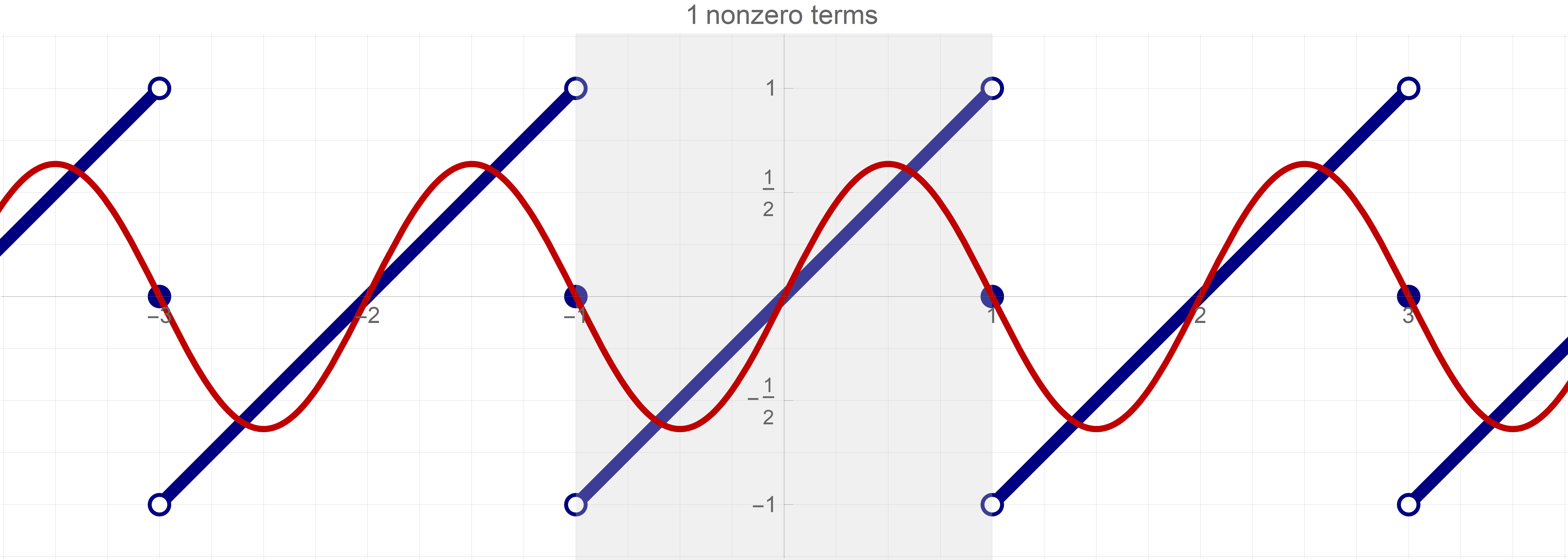
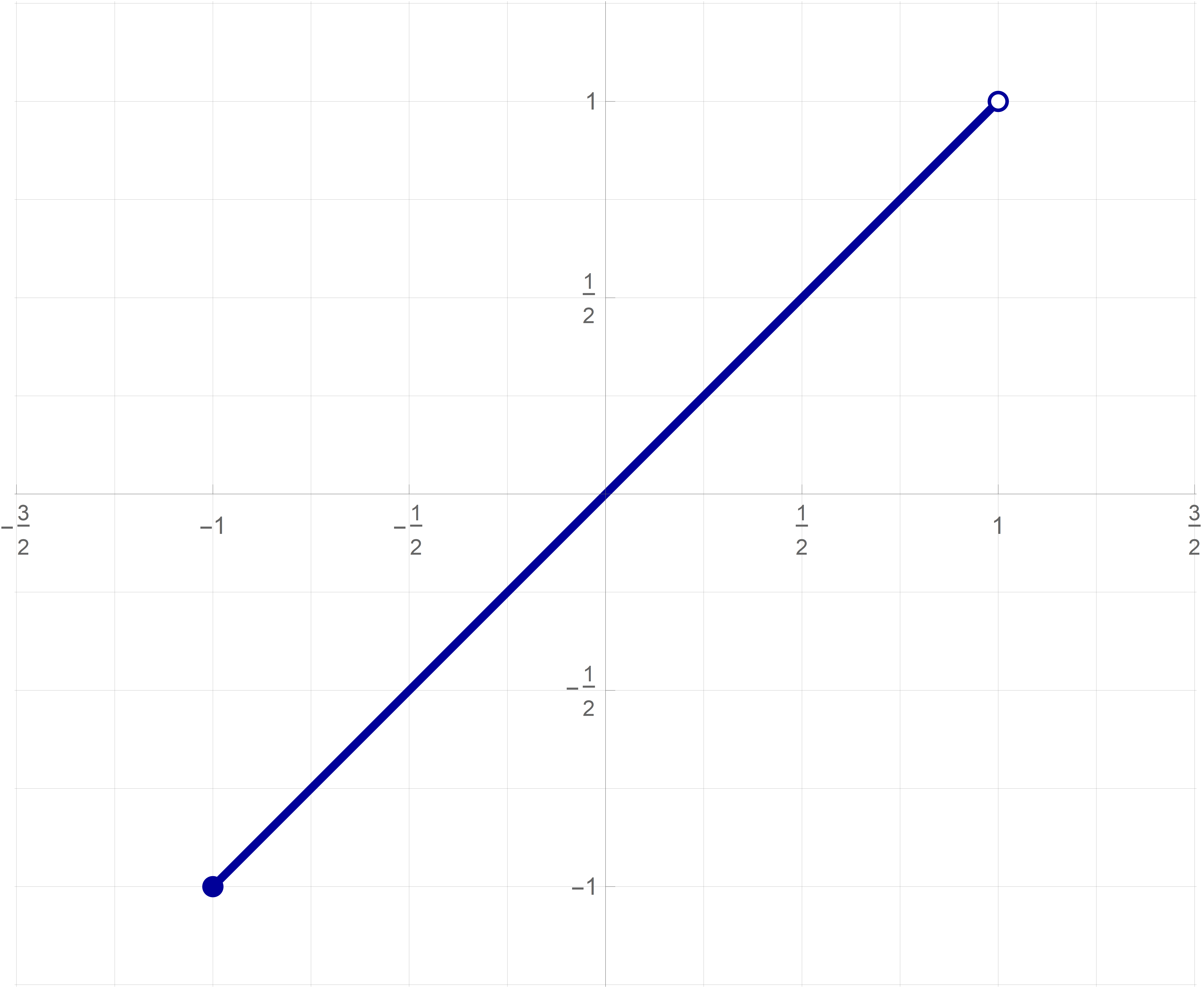
Yesterday we calculated the Fourier Series for the function \( f(x) = x\) with \(x\in [-1,1) \). The Fourier series is given by the formula below, and it converges to the Fourier periodic extension of the function \(f\): \[ \tilde{f}_{\!\operatorname{Fourier}}(x) = \frac{2}{\pi} \sum_{k=1}^\infty \frac{(-1)^{k+1}}{k} \sin(\pi k x). \] We illustrated the relationship between partial sums of this Fourier series and the Fourier periodic extension of $f$ in the plots below.
The plots below, represent the Fourier periodic extension of $f$ in navy blue and different partial sums of the Fourier series in red.
Click on the image below to cycle through different versions.
- The question that we want to answer here is as follows: Find the function \(v(x)\) defined on \([-1,1)\) whose Fourier series is \[ \sum_{k=1}^\infty \frac{1}{k}\mkern 2mu \sin(\pi k x). \]
-
The idea here is to modify the formula
\[
\tilde{f}_{\!\operatorname{Fourier}}(x) = \frac{2}{\pi} \sum_{k=1}^\infty \frac{(-1)^{k+1}}{k} \sin(\pi k x)
\]
to get
\[
\sum_{k=1}^\infty \frac{1}{k}\mkern 2mu \sin(\pi k x).
\]
on the right-hand side.
- First we multiply by \(\dfrac{\pi}{2}\) the Fourier series for \(f\): \[ \dfrac{\pi}{2} \tilde{f}_{\!\operatorname{Fourier}}(x) = \sum_{k=1}^\infty \frac{(-1)^{k+1}}{k} \sin(\pi k x). \]
- Next we recognize that \((-1)^k = \cos(k \pi)\). Therefore \begin{align*} (-1)^k \sin(\pi k x) & = \sin(\pi k x) \mkern 2mu \cos(k \pi) \\ \fbox{since \(\ \sin(k \pi) = 0\)} & = \sin(k \pi x) \mkern 2mu \cos(k \pi) + \cos(k \pi x) \mkern 2mu \sin(k \pi) \\ \fbox{\(\sin(\alpha+\beta) = ... \)} & = \sin\bigl(k\pi (x+1) \bigr). \end{align*} See the link \(\sin(\alpha+\beta) = ... \) for the complete formula. Consequently, \[ \dfrac{\pi}{2} \tilde{f}_{\!\operatorname{Fourier}}(x) = - \sum_{k=1}^\infty \frac{1}{k} \sin\bigl(k \pi (x+1)\bigr). \]
- Multiplying the last formula from the preceding ➢ item with \(-1\) and changing variable \(x+1\) to \(t\), and therefore \(x\) to \(t-1\) we get \[ - \dfrac{\pi}{2} \tilde{f}_{\!\operatorname{Fourier}}(t-1) = \sum_{k=1}^\infty \frac{1}{k} \sin\bigl(k \pi t\bigr). \] But, we are used for the independent variable to be called \(x\), so we rewrite the last Fourier series as \[ \sum_{k=1}^\infty \frac{1}{k} \sin\bigl(k \pi x \bigr) = - \dfrac{\pi}{2} \tilde{f}_{\!\operatorname{Fourier}}(x-1). \]
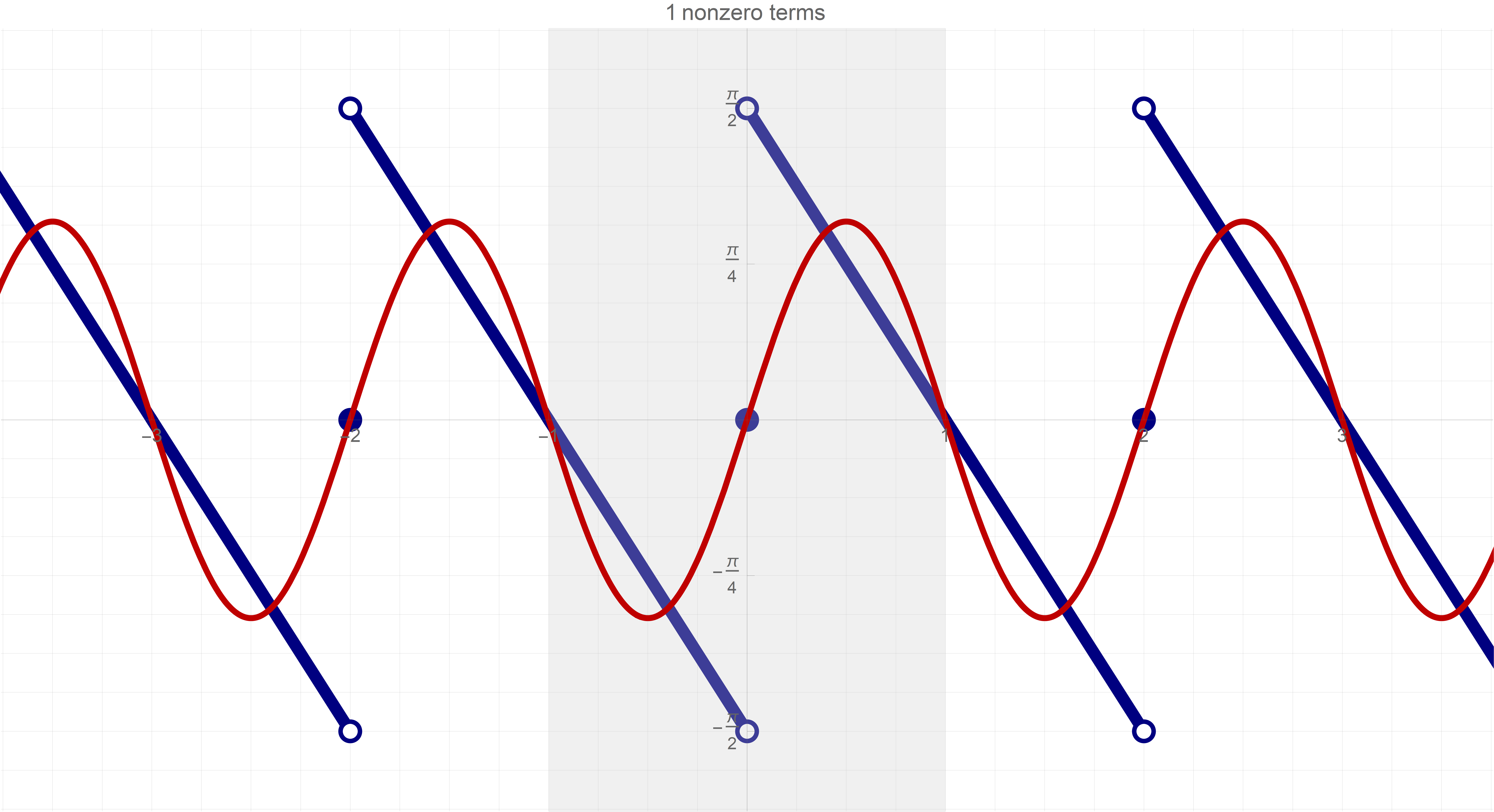
- Next we need to figure out the formula for \[ - \dfrac{\pi}{2} \tilde{f}_{\!\operatorname{Fourier}}(x-1) \] on \([-1,1)\). That is the function \(v(x)\) that we seek. Recall that the change of the independent variable \(x-1\) shifts the graph by \(1\) unit to the right, multiplication by \(\dfrac{\pi}{2}\) scales the graph and multiplication by \(-1\) flips the graph accross \(x\)-axis. This process is easier by drawing plots. We figure out the piecewise formula for \(v\) is \[ v(x) = \begin{cases} - \dfrac{\pi}{2} (x+1) & \text{if} \ x \in [-1,0), \\[4pt] 0 & \text{if} \ x = 0, \\[4pt] - \dfrac{\pi}{2} (x-1) & \text{if} \ x \in (0,1]. \end{cases} \] Using the Sign Function we can write \[ v(x) = \dfrac{\pi}{2} \bigl( \operatorname{sgn}(x) - x \bigr), \quad x \in [-1,1). \]
-
The plots below, represent the Fourier periodic extension of $v$ in navy blue and different partial sums of its Fourier series in red.
Click on the image below to cycle through different versions.
-
Recall the definition of a Fourier series:
Definition. Let $L \gt 0$ and let $f:[-L, L] \to \mathbb R$ be a piecewise continuous function. The series \[ a_0 + \sum_{k=1}^{+\infty} \biggl( a_k \cos\Bigl(\!\frac{k \pi}{L} x\!\Bigr) + b_k \sin\Bigl(\!\frac{k \pi}{L} x\!\Bigr) \biggr) \] where \[ a_0 = \frac{1}{2L} \int_{-L}^L f(\xi) d\xi \] and, for $k \in {\mathbb N}$, \begin{align*} a_k &= \frac{1}{L}\int_{-L}^L f(\xi) \cos\Bigl(\!\frac{k \pi}{L} \xi\!\Bigr) d\xi, \\ b_k &= \frac{1}{L}\int_{-L}^L f(\xi) \sin\Bigl(\!\frac{k \pi}{L} \xi\!\Bigr) d\xi, \end{align*} is called the Fourier series of $f$.
-
Recall the definition of the Fourier periodic extension of $f:[-L, L] \to \mathbb R$.
Definition of Fourier Periodic Extension. Let $L \gt 0$ and \[ f:[-L, L] \to \mathbb R \] be a piecewise continuous function. Then the Periodic Extension of \(f:[-L,L) \to \mathbb{R}\) is the following function defined for all \(x\in \mathbb{R}\) by \[ \widetilde{\mkern3mu f\mkern 1mu}(x) = f\biggl(x - 2 L \Bigl\lfloor \frac{x+L}{2L}\Bigr\rfloor \biggr). \] The Fourier periodic extension of $f$ is the following function defined for all \(x\in \mathbb{R}\) by \[ \tilde{f}_{\!\operatorname{Fourier}}(x) = \begin{cases} \tilde{f}(x) & \text{if $\tilde{f}$ is continuous at $x$} \\[10pt] \dfrac{1}{2}\!\bigl(\tilde{f}(x^-)+\tilde{f}(x^+)\bigr) & \text{if $\tilde{f}$ is not continuous at $x$} \end{cases} \] where \[ \tilde{f}(x^-) = \lim_{\xi \uparrow x} \tilde{f}(\xi) \quad \text{left-hand limit} \] and \[ \tilde{f}(x^+) = \lim_{\xi \downarrow x} \tilde{f}(\xi) \quad \text{right-hand limit}. \]
-
Recall the convergence theorems:
- Pointwise Convergence Theorem. If $f$ is piecewise smooth on $[-L,L]$, then for every $x \in {\mathbb R}$ we have \[ \lim_{n \to +\infty} S_n^f(x) = \tilde{f}_{\!\operatorname{Fourier}}(x). \] Loosely speaking, the Fourier series of $f$ converges pointwise to the Fourier periodic extension of $f$.
- Notice that if the periodic extension of $f$ is a continuous function, then the Fourier periodic extension of $f$ coincides with the periodic extension of $f$. In other words, if $\tilde{f}$ is a continuous function, then $\tilde{f}_{\!\!\rm Fourier} = \tilde{f}$.
- Uniform Convergence Theorem. If $f$ is piecewise smooth and the periodic extension of $f$ is continuous, then the sequence of functions $\bigl\{S_n^f\bigr\}_{n=1}^{+\infty}$ converges uniformly on ${\mathbb R}$ to $\tilde{f}$. This means that for every $\varepsilon > 0$ there exists $N_\epsilon \in \mathbb{R}$ such that for all $n \gt N_\varepsilon$ and for all $x \in {\mathbb R}$ we have \[ \Bigl|S_n^f(x) - \tilde{f}(x) \Bigr| < \varepsilon. \]
-
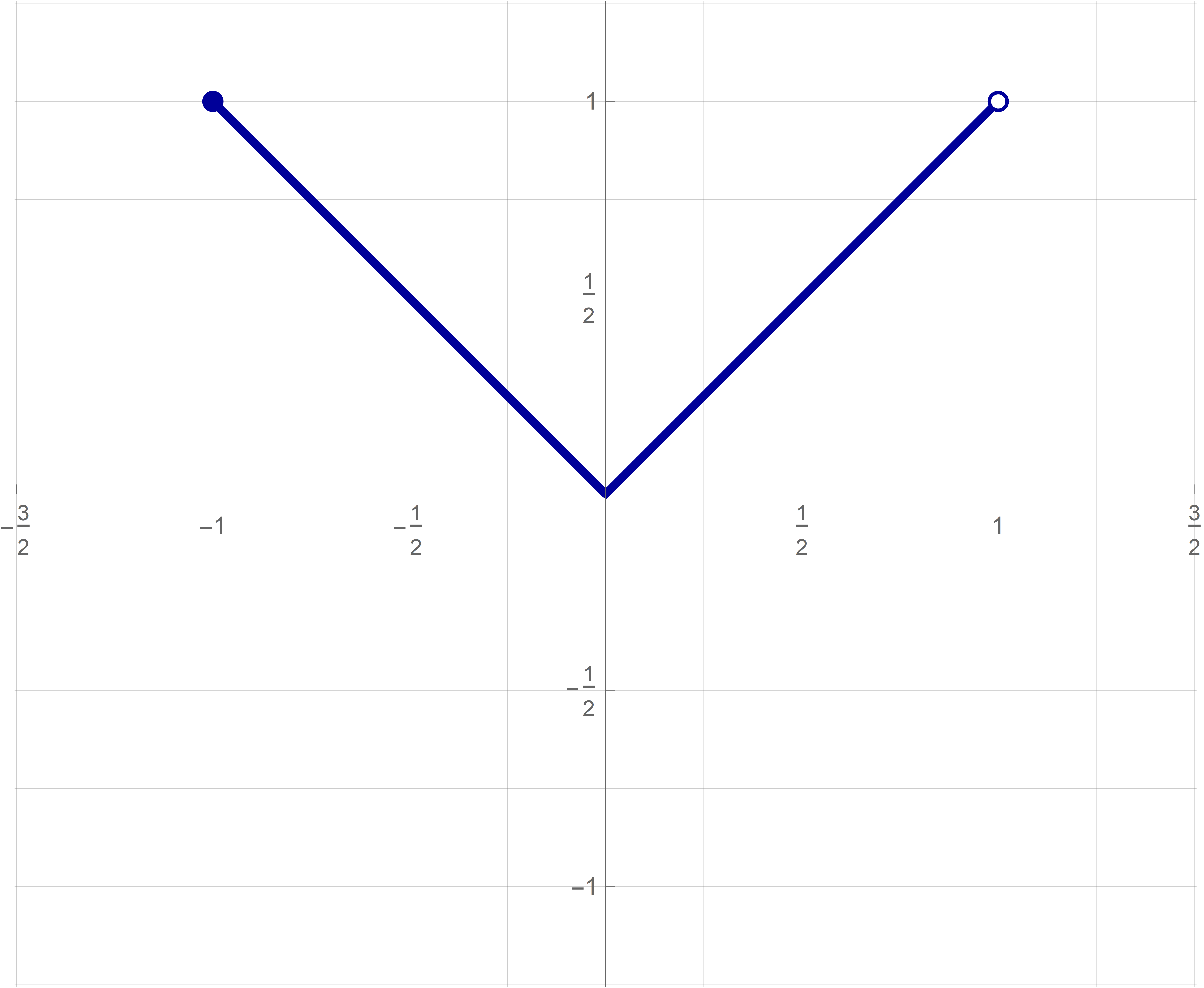
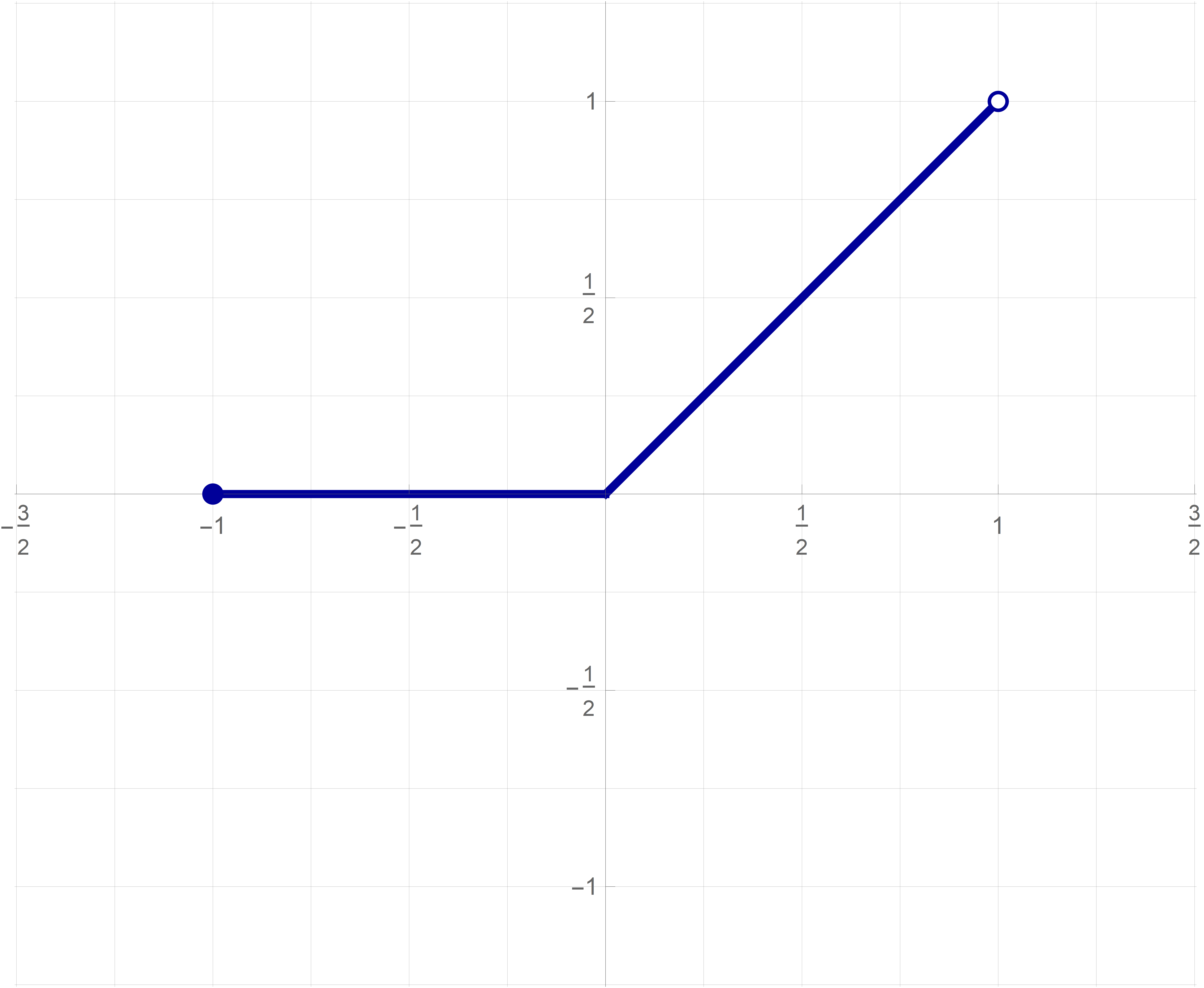
In the rest of today's post we will study the Fourier series of the following three functions:
Function: \( f(x) = x\) with \(x\in [-1,1) \) Function: \( g(x) = |x|\) with \(x\in [-1,1) \) Function: \( h(x) = \operatorname{ReLU}(x) \) with \(x\in [-1,1) \) - First notice that the function \(f\) is odd and the function \(g\) is even.
- These three functions are clearly related to each other. The average of \(f\) and \(g\) is \(h\): \[ h(x) = \frac{1}{2} f(x) + \frac{1}{2} g(x). \] Replacing in the preceding equality \(x\) by \(-x\) and using that \(f(-x) = - f(x)\) and \(g(-x) = g(x)\) we get \[ h(-x) = - \frac{1}{2} f(x) + \frac{1}{2} g(x). \]
- First adding, and than subtracting the displayed equalities in the previous ➢ item, we obtain \[ g(x) = h(x) + h(-x), \] and \[ f(x) = h(x) - h(-x). \]
- To calculate the coefficients of the Fourier series of the given three functions we will need the following two indefinite integrals (here \(k \in \mathbb{N}\)) \begin{align*} \int x \cos(k \pi x) \operatorname{d}\mkern-3mu x & = \frac{\cos (\pi k x)}{\pi ^2 k^2}+\frac{x \sin (\pi k x)}{\pi k} \\[6pt] \int x \sin(k \pi x) \operatorname{d}\mkern-3mu x & = \frac{\sin (\pi k x)}{\pi ^2 k^2}-\frac{x \cos (\pi k x)}{\pi k} \end{align*}
-
The Fourier Series for the function \( f(x) = x\) with \(x\in [-1,1) \).
- The function \(f\) is odd. Therefore the coefficient \[ a_0 = \frac{1}{2} \int_{-1}^1 \xi \operatorname{d}\mkern-3mu\xi = 0 \] and for all \(k\in\mathbb{N}\) \[ a_k = \frac{1}{1} \int_{-1}^1 \xi \cos(\pi k \xi) \operatorname{d}\mkern-3mu\xi = 0. \]
- Using the above given indefinite integrals and the Fundamental Theorem of Calculus, for the coefficients \(b_k\) we have \[ b_k = \frac{1}{1} \int_{-1}^1 \xi \sin(\pi k \xi) \operatorname{d}\mkern-3mu\xi = \frac{2}{\pi} \frac{(-1)^{k+1}}{k} \]
- Thus the Fourier Series for the function \( f(x) = x\) with \(x\in [-1,1) \) is \[ \frac{2}{\pi} \sum_{k=1}^\infty \frac{(-1)^{k+1}}{k} \sin(\pi k x). \] Since the function \(f\) is piecewise smooth, the pointwise convergence theorem implies that this Fourier series converges to the Fourier periodic extension of $f$. That is, for every \(x\in \mathbb{R}\) we have \[ \tilde{f}_{\!\operatorname{Fourier}}(x) = \frac{2}{\pi} \sum_{k=1}^\infty \frac{(-1)^{k+1}}{k} \sin(\pi k x). \]
-
The plots below, represent the Fourier periodic extension of $f$ in navy blue and different partial sums of the Fourier series in red.
Click on the image below to cycle through different versions.
- Since in this case the Fourier periodic extension of $f$ is simple, we can state the convergence explicitly: \[ \forall \mkern 2mu x \in (-1,1) \qquad x = \frac{2}{\pi} \sum_{k=1}^\infty \frac{(-1)^{k+1}}{k} \sin(\pi k x). \]
- The last formula in the preceding ➢ item, when specialized to \(x = 1/2\), gives: \[ \frac{1}{2} = \frac{2}{\pi} \sum_{k=1}^\infty \frac{(-1)^{k+1}}{k} \sin\Bigl(\pi k \frac{1}{2}\Bigr). \] Since for even \(k\) we have \(\sin\Bigl(\pi k \frac{1}{2}\Bigr) = 0\), the last displayed formula simplifies to \[ \frac{\pi}{4} = \sum_{m=1}^\infty \frac{1}{2m-1} \sin\Bigl(\pi (2m-1) \frac{1}{2}\Bigr). \] Since for \(m\in\mathbb{N}\) we have \[ \sin\Bigl(\pi (2m-1) \frac{1}{2}\Bigr) = (-1)^{m+1}, \] we finally get \[ \frac{\pi}{4} = \sum_{m=1}^\infty \frac{(-1)^{m+1}}{2m-1} = 1 -\frac{1}{3} + \frac{1}{5} - \frac{1}{7} - \frac{1}{9} + \cdots \] This formula has interesting history, see Madhava Series - Wikipedia and Leibniz Formula - Wikipedia.
-
The Fourier Series for the function \( g(x) = |x|\) with \(x\in [-1,1) \).
- The function \(g\) is even. Therefore the coefficient \[ a_0 = \frac{1}{2} \int_{-1}^1 |\xi| \operatorname{d}\mkern-3mu\xi = \frac{1}{2} 2 \int_{0}^1 \xi \operatorname{d}\mkern-3mu\xi = \frac{1}{2} \] and for all \(k\in\mathbb{N}\), using the above given indefinite integrals and the Fundamental Theorem of Calculus, for the coefficients \(a_k\) we have \[ a_k = \frac{1}{1} 2 \int_{0}^1 \xi \cos(\pi k \xi) \operatorname{d}\mkern-3mu\xi = \frac{2 \left((-1)^k-1\right)}{\pi ^2 k^2}. \] Thus, all even indexed coefficients are equal to \(0\), and for odd indexed coefficients we have \[ a_{2m-1} = - \frac{4}{\pi ^2} \frac{1}{(2m-1)^2}. \]
- Since the function \(g\) is even all coefficients \(b_k = 0\).
- Thus the Fourier Series for the function \( g(x) = |x|\) with \(x\in [-1,1) \) is \[ \frac{1}{2} - \frac{4}{\pi ^2} \sum_{m=1}^\infty \frac{1}{(2m-1)^2} \cos\bigl((2 m - 1) \pi x\bigr). \] Since the periodic extension of function \(g\) is continuous and piecewise smooth, the uniform convergence theorem implies that this Fourier series converges to the continuous periodic extension of $g$. That is, for every \(x\in \mathbb{R}\) we have \[ \tilde{g}(x) =\frac{1}{2} - \frac{4}{\pi ^2} \sum_{m=1}^\infty \frac{1}{(2m-1)^2} \cos\bigl((2 m - 1) \pi x\bigr). \]
-
The plots below, represent the periodic extension of $g$ in navy blue and different partial sums of the Fourier series in red.
Click on the image below to cycle through different versions.
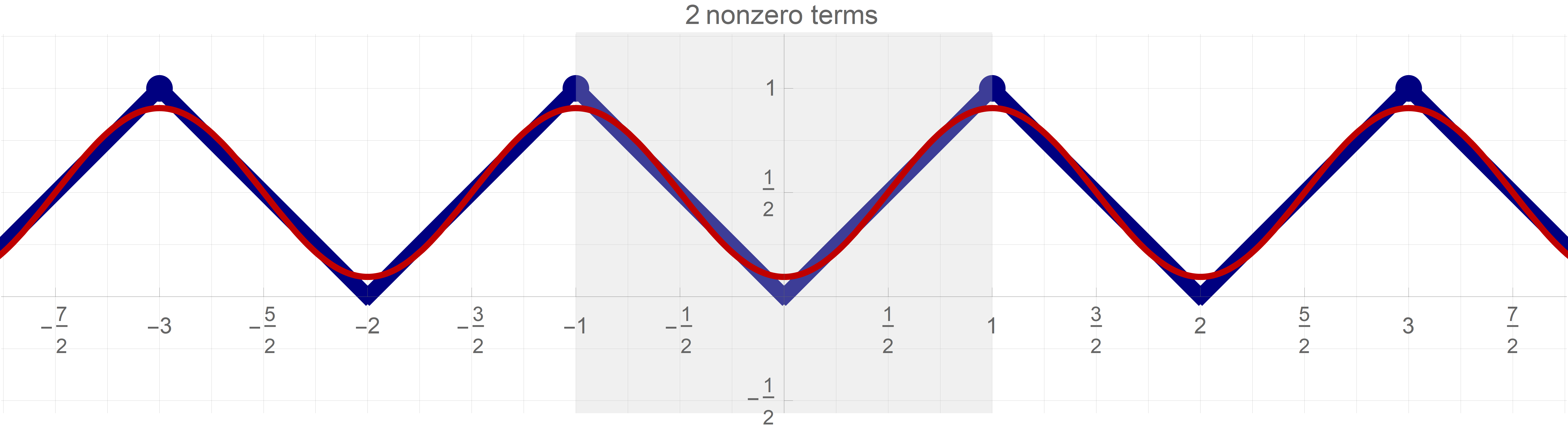
- Since in this case the periodic extension of $f$ is simple, we can state the convergence explicitly: \[ \forall \mkern 2mu x \in [-1,1] \qquad |x| = \frac{1}{2} - \frac{4}{\pi ^2} \sum_{m=1}^\infty \frac{1}{(2m-1)^2} \cos\bigl((2 m - 1) \pi x\bigr). \]
- The last formula in the preceding ➢ item, when specialized to \(x = 1\), gives: \[ 1 = \frac{1}{2} - \frac{4}{\pi ^2} \sum_{m=1}^\infty \frac{1}{(2m-1)^2} \cos\bigl((2 m - 1) \pi\bigr). \] Since \(\cos\bigl((2 m - 1) \pi\bigr) = -1\), the last displayed formula simplifies to \[ \frac{\pi ^2}{8} = \sum_{m=1}^\infty \frac{1}{(2m-1)^2}. \] This formula is a part of the Basel Problem - Wikipedia to calculate \[ S = \sum_{n=1}^\infty \frac{1}{n^2}. \] We calculate \(S\) based on the series that we already calculated: \begin{align*} S & = \sum_{n=1}^\infty \frac{1}{n^2} \\ & = \sum_{m=1}^\infty \frac{1}{(2m-1)^2} + \sum_{m=1}^\infty \frac{1}{(2m)^2} \\ & = \frac{\pi ^2}{8} + \frac{1}{4} \sum_{m=1}^\infty \frac{1}{m^2} \\ & = \frac{\pi ^2}{8} + \frac{1}{4} S. \end{align*} Hence \[ \frac{3}{4} S = \frac{\pi ^2}{8}, \] that is \[ S = \frac{\pi ^2}{6}. \]
-
The Fourier Series for the function \( h(x) = x \operatorname{us}(x)\) with \(x\in [-1,1) \).
- Since we established that \[ h(x) = \frac{1}{2} g(x) + \frac{1}{2} f(x), \] from the previous calculations we have that the Fourier series for the function \(h\) is \begin{align*} \frac{1}{4} - \frac{2}{\pi ^2} \sum_{m=1}^\infty \frac{1}{(2m-1)^2} & \cos\bigl((2 m - 1) \pi x\bigr) \\ & + \frac{1}{\pi} \sum_{k=1}^\infty \frac{(-1)^{k+1}}{k} \sin(\pi k x). \end{align*} Since the periodic extension of function \(h\) is piecewise smooth, the pointwise convergence theorem implies that this Fourier series converges to the Fourier periodic extension of $h$. That is, for every \(x\in \mathbb{R}\) we have \begin{align*} \tilde{h}(x) = \frac{1}{4} - \frac{2}{\pi ^2} \sum_{m=1}^\infty \frac{1}{(2m-1)^2} & \cos\bigl((2 m - 1) \pi x\bigr) \\ & + \frac{1}{\pi} \sum_{k=1}^\infty \frac{(-1)^{k+1}}{k} \sin(\pi k x). \end{align*}
-
The plots below, represent the Fourier periodic extension of \(h\) in navy blue and different partial sums of its Fourier series in red.
Click on the image below to cycle through different versions.
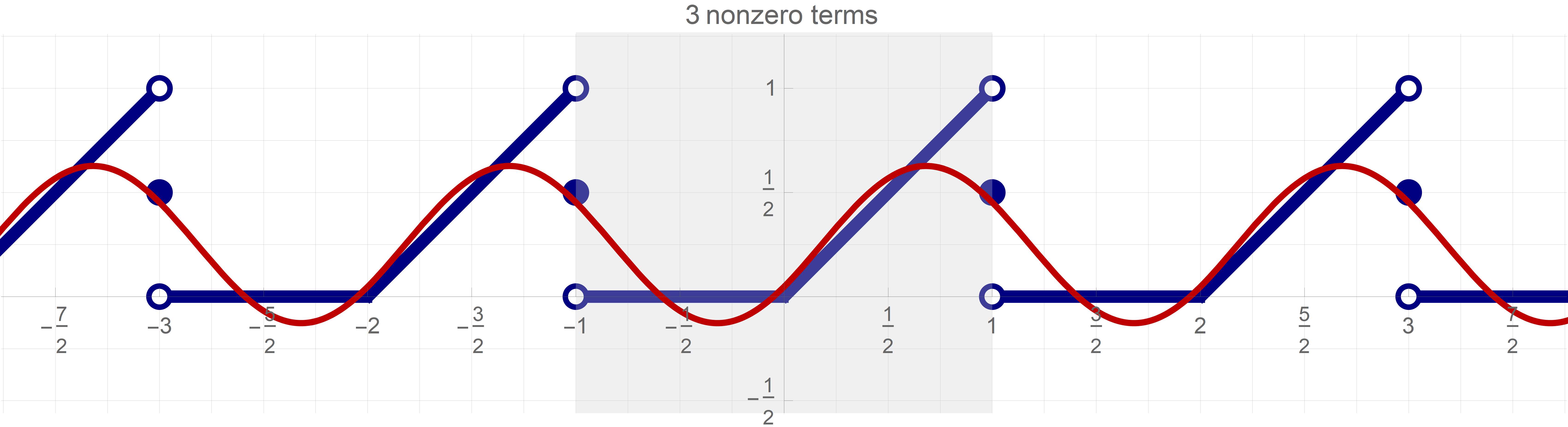
- Since in this case the Fourier periodic extension of $h$ is relatively simple, we can state the convergence explicitly: \begin{align*} \frac{1}{4} - \frac{2}{\pi ^2} \sum_{m=1}^\infty & \frac{1}{(2m-1)^2} \cos\bigl((2 m - 1) \pi x\bigr) \\ & + \frac{1}{\pi} \sum_{k=1}^\infty \frac{(-1)^{k+1}}{k} \sin(\pi k x) = \begin{cases} \frac{1}{2} & \text{if} \ \ x \in \{-1,1\}, \\[6pt] 0 & \text{if} \ \ x \in (-1,0), \\[6pt] x & \text{if} \ \ x \in [0,1). \end{cases} \end{align*}
- Can the last expression be specialized to some \(x\in [-1,1]\) to get some interesting numerical series?
- Today we discussed Fourier series of a piecewise smooth function. The relevant sections are Section 3.1 and Section 3.2: the assigned problems are 3.2.1, 3.2.2, 3.2.3, 3.2.4.
- Also, see my webpage Fourier periodic extension.
-
- Definition. Let $L \gt 0$ and let $f:[-L, L] \to \mathbb R$ be a piecewise continuous function. The series \[ a_0 + \sum_{k=1}^{+\infty} \biggl( a_k \cos\Bigl(\!\frac{k \pi}{L} x\!\Bigr) + b_k \sin\Bigl(\!\frac{k \pi}{L} x\!\Bigr) \biggr) \] where \[ a_0 = \frac{1}{2L} \int_{-L}^L f(\xi) d\xi \] and, for $k \in {\mathbb N}$, \begin{align*} a_k &= \frac{1}{L}\int_{-L}^L f(\xi) \cos\Bigl(\!\frac{k \pi}{L} \xi\!\Bigr) d\xi, \\ b_k &= \frac{1}{L}\int_{-L}^L f(\xi) \sin\Bigl(\!\frac{k \pi}{L} \xi\!\Bigr) d\xi, \end{align*} is called the Fourier series of $f$.
-
To understand the convergence of the Fourier series of a function $f:[-L,L] \to \mathbb{R}$ we first need to define the concept of a piecewise smooth function and its periodic extension. This is studied in Chapter 3 in the textbook. However, the book does not have formal definitions of piecewise smooth function and its periodic extension. Therefore, I give a few formal definitions here.
-
Definition.
Let $a$ and $b$ be real numbers such that $a \lt b$. A function $f:[a,b] \to \mathbb R$ is said to be piecewise continuous on $[a,b]$ if the following conditions are satisfied:
- there exists a finite set $\{x_1,\ldots,x_n\} \subset (a,b)$ such that $x_1 \lt \cdots \lt x_n$ and $f$ is continuous on each interval \[ (a,x_1), \quad (x_k,x_{k+1}), \ \ k \in \{1,\ldots,n-1\}, \quad (x_n,b); \]
- all the following one-sided limits exist \[ \lim_{x\downarrow a} f(x), \quad \lim_{x\uparrow x_k} f(x), \quad \lim_{x\downarrow x_k} f(x), \ k \in \{1,\ldots,n\}, \quad \lim_{x\uparrow b} f(x). \]
-
Definition. Let $a$ and $b$ be real numbers such that $a \lt b$. A function $f:[a,b] \to \mathbb R$ is said to be piecewise smooth on $[a,b]$ if the following conditions are satisfied:
- there exists a finite set $\{x_1,\ldots,x_n\} \subset (a,b)$ such that $x_1 \lt \cdots \lt x_n$ and $f$ is continuous and it has a continuous derivative $f'$ on each interval \[ (a,x_1), \quad (x_k,x_{k+1}), \ k \in \{1,\ldots,n-1\}, \quad (x_n,b); \]
- all the following one-sided limits exist \[ \lim_{x\downarrow a} f(x), \quad \lim_{x\uparrow x_k} f(x), \quad \lim_{x\downarrow x_k} f(x), \ k \in \{1,\ldots,n\}, \quad \lim_{x\uparrow b} f(x); \]
- all the following one-sided limits exist \[ \lim_{x\downarrow a} f'(x), \quad \lim_{x\uparrow x_k} f'(x), \quad \lim_{x\downarrow x_k} f'(x), \ k \in \{1,\cdots,n\}, \quad \lim_{x\uparrow b} f'(x). \]
- Definition. Let $a$ and $b$ be real numbers such that $a \lt b$ and let $f:(a,b] \to \mathbb R$ be a function. The function $\tilde{f}: {\mathbb R} \to {\mathbb R}$ defined by \[ \tilde{f}(x) = f\left(\!x-\left\lceil\!\dfrac{x-b}{b-a}\! \right\rceil (b-a)\!\right), \quad x \in {\mathbb R}. \] is called the periodic extension of $f$.
- Definition. Let $a$ and $b$ be real numbers such that $a \lt b$ and let $f:[a,b) \to \mathbb R$ be a function. The function $\tilde{f}: {\mathbb R} \to {\mathbb R}$ defined by \[ \tilde{f}(x) = f\left(\!x- \left\lfloor\!\dfrac{x-a}{b-a}\! \right\rfloor (b-a)\!\right), \quad x \in {\mathbb R}. \] is called the periodic extension of $f.$
- For the explanation of these definitions see my webpage Fourier periodic extension.
-
Definition.
Let $a$ and $b$ be real numbers such that $a \lt b$. A function $f:[a,b] \to \mathbb R$ is said to be piecewise continuous on $[a,b]$ if the following conditions are satisfied:
-
I do understand that the last two definitions might look somewhat weird. The only reason for that is that the ceiling function and the floor function are almost completely absent from our curriculum. That is a fault of our curriculum.
The floor function is defined as follows: For $x \in \mathbb{R}$ we set \[ \lfloor x \rfloor = \max \bigl\{ k \in \mathbb{Z} : k \leq x \bigr\}. \] In words: The floor function of a real number $x$ is defined as the largest integer less than or equal to $x$. This means it rounds $x$ down to the nearest integer. For example, $\lfloor \pi \rfloor = 3$, $\lfloor -e \rfloor = -3$.
The ceiling function is defined as follows: For $x \in \mathbb{R}$ we set \[ \lceil x \rceil = \min \bigl\{ k \in \mathbb{Z} : x \leq k \bigr\}. \] In words: The ceiling function of a real number $x$ is the smallest integer greater than or equal to $x$. This means it rounds $x$ up to the nearest integer. For example, $\lceil \pi \rceil = 4$, $\lceil -e \rceil = -2$.
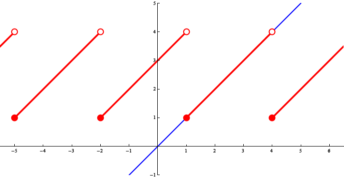
The book gives a descriptive definition in English of the concept of a periodic extension. The above formula involving the ceiling and floor function is the only way that I was able to translate the definition from English into Mathish. The figures below illustrate the definition with some simple functions $f$. Here is the Mathematica notebook which I used to produce these figures.
In the figure below the function $f$ is the restriction of the function $x \mapsto x$ (in blue) to the interval $[1,4)$. The red function is the periodic extension.
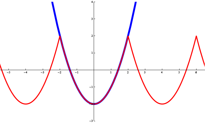
In the figure below the function $f$ is the restriction of the function $x \mapsto x^2-2$ (in blue) to the interval $[-2,2)$. The red function is the periodic extension.
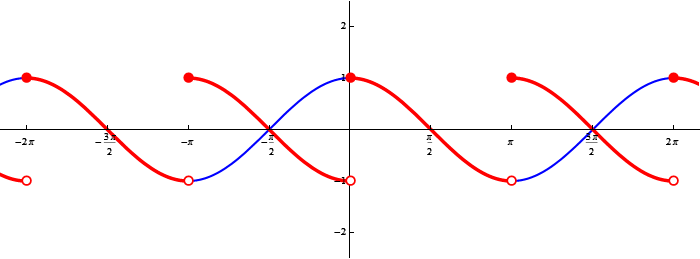
In the figure below the function $f$ is the restriction of the function $x \mapsto \cos(x)$ (in blue) to the interval $[0,\pi)$. The red function is the periodic extension.
- Read Section 3.1 and Section 3.2 in the book. This is a small notebook that I wrote in class today.
-
Yesterday, we discussed Fourier series of a piecewise smooth function. The relevant sections are Section 3.1 and Section 3.2: the assigned problems are 3.2.1, 3.2.2, 3.2.3, 3.2.4. Some of the content is on my webpage Fourier periodic extension.
- Definition. Let $L \gt 0$ and let $f:[-L, L] \to \mathbb R$ be a piecewise continuous function. The series \[ a_0 + \sum_{k=1}^{+\infty} \biggl( a_k \cos\Bigl(\!\tfrac{k \pi}{L} x\!\Bigr) + b_k \sin\Bigl(\!\tfrac{k \pi}{L} x\!\Bigr) \biggr) \] where \[ a_0 = \frac{1}{2L} \int_{-L}^L f(\xi) d\xi \] and, for $k \in {\mathbb N}$, \begin{align*} a_k &= \frac{1}{L}\int_{-L}^L f(\xi) \cos\Bigl(\!\tfrac{k \pi}{L} \xi\!\Bigr) d\xi, \\ b_k &= \frac{1}{L}\int_{-L}^L f(\xi) \sin\Bigl(\!\tfrac{k \pi}{L} \xi\!\Bigr) d\xi, \end{align*} is called the Fourier series of $f$.
-
To understand the convergence of the Fourier series of a function $f:[-L,L] \to \mathbb{R}$ we first need to define the concept of a piecewise smooth function and its periodic extension. This is studied in Chapter 3 in the textbook. However, the book does not have formal definitions of piecewise smooth function and its periodic extension. Therefore, I give few formal definitions here. For more see my webpage about
Fourier periodic extension.
-
Definition.
Let $a$ and $b$ be real numbers such that $a \lt b$. A function $f:[a,b] \to \mathbb R$ is said to be piecewise continuous on $[a,b]$ if the following conditions are satisfied:
- there exists a finite set $\{x_1,\ldots,x_n\} \subset (a,b)$ such that $x_1 \lt \cdots \lt x_n$ and $f$ is continuous on each interval \[ (a,x_1), \quad (x_k,x_{k+1}), \ \ k \in \{1,\ldots,n-1\}, \quad (x_n,b); \]
- all the following one-sided limits exist \[ \lim_{x\downarrow a} f(x), \quad \lim_{x\uparrow x_k} f(x), \quad \lim_{x\downarrow x_k} f(x), \ k \in \{1,\ldots,n\}, \quad \lim_{x\uparrow b} f(x). \]
-
Definition. Let $a$ and $b$ be real numbers such that $a \lt b$. A function $f:[a,b] \to \mathbb R$ is said to be piecewise smooth on $[a,b]$ if the following conditions are satisfied:
- there exists a finite set $\{x_1,\ldots,x_n\} \subset (a,b)$ such that $x_1 \lt \cdots \lt x_n$ and $f$ is continuous and it has a continuous derivative $f'$ on each interval \[ (a,x_1), \quad (x_k,x_{k+1}), \ k \in \{1,\ldots,n-1\}, \quad (x_n,b); \]
- all the following one-sided limits exist \[ \lim_{x\downarrow a} f(x), \quad \lim_{x\uparrow x_k} f(x), \quad \lim_{x\downarrow x_k} f(x), \ k \in \{1,\ldots,n\}, \quad \lim_{x\uparrow b} f(x); \]
- all the following one-sided limits exist \[ \lim_{x\downarrow a} f'(x), \quad \lim_{x\uparrow x_k} f'(x), \quad \lim_{x\downarrow x_k} f'(x), \ k \in \{1,\cdots,n\}, \quad \lim_{x\uparrow b} f'(x). \]
- Definition. Let $a$ and $b$ be real numbers such that $a \lt b$ and let $f:(a,b] \to \mathbb R$ be a function. The function $\tilde{f}: {\mathbb R} \to {\mathbb R}$ defined by \[ \tilde{f}(x) = f\left(\!x-\left\lceil\!\dfrac{x-b}{b-a}\! \right\rceil (b-a)\!\right), \quad x \in {\mathbb R}. \] is called the periodic extension of $f$.
- Definition. Let $a$ and $b$ be real numbers such that $a \lt b$ and let $f:[a,b) \to \mathbb R$ be a function. The function $\tilde{f}: {\mathbb R} \to {\mathbb R}$ defined by \[ \tilde{f}(x) = f\left(\!x- \left\lfloor\!\dfrac{x-a}{b-a}\! \right\rfloor (b-a)\!\right), \quad x \in {\mathbb R}. \] is called the periodic extension of $f.$
- Explanation. The reasoning for the above definition of the periodic extension is as follows. For every $x\in\mathbb R$ there exists unique $k \in \mathbb Z$ such that \[ a + k (b-a) \leq x \lt a + (k+1)(b-a). \] The last expression is equivalent to \[ k \leq \frac{x - a}{b-a} \lt k+1. \] Therefore \[ k = \left\lfloor \frac{x - a}{b-a} \right\rfloor. \] Consequently \[ x - \left\lfloor\!\dfrac{x-a}{b-a} \right\rfloor(b-a) \in [a,b). \]
-
Definition.
Let $a$ and $b$ be real numbers such that $a \lt b$. A function $f:[a,b] \to \mathbb R$ is said to be piecewise continuous on $[a,b]$ if the following conditions are satisfied:
-
I do understand that the last two definitions might look somewhat weird. The only reason for that is that the ceiling function and the floor function are almost completely absent from our curriculum. That is a fault of our curriculum.
The floor function is defined as follows: For $x \in \mathbb{R}$ we set \[ \lfloor x \rfloor = \max \bigl\{ k \in \mathbb{Z} : k \leq x \bigr\}. \] In words: The floor function of a real number $x$ is defined as the largest integer less than or equal to $x$. This means it rounds $x$ down to the nearest integer. For example, $\lfloor \pi \rfloor = 3$, $\lfloor -e \rfloor = -3$.
The ceiling function is defined as follows: For $x \in \mathbb{R}$ we set \[ \lceil x \rceil = \min \bigl\{ k \in \mathbb{Z} : x \leq k \bigr\}. \] In words: The ceiling function of a real number $x$ is the smallest integer greater than or equal to $x$. This means it rounds $x$ up to the nearest integer. For example, $\lceil \pi \rceil = 4$, $\lceil -e \rceil = -2$.
The book gives a descriptive definition in English of the concept of a periodic extension. The above formula involving the ceiling and floor function is the only way that I was able to translate the definition from English into Mathish. The figures below illustrate the definition with some simple functions $f$. Here is the Mathematica notebook which I used to produce these figures.
In the figure below the function $f$ is the restriction of the function $x \mapsto x$ (in blue) to the interval $[1,4)$. The red function is the periodic extension.
In the figure below the function $f$ is the restriction of the function $x \mapsto x^2-2$ (in blue) to the interval $[-2,2)$. The red function is the periodic extension.
In the figure below the function $f$ is the restriction of the function $x \mapsto \cos(x)$ (in blue) to the interval $[0,\pi)$. The red function is the periodic extension.
- Read Section 3.1 and Section 3.2 in the book.
- I post two Mathematica notebooks and their pdf printouts. A prudent practice in working with Mathematica notebooks is to before saving a notebook. is an item in the menu list . After you it is a good idea to (this will evaluate the entire notebook), in the menu list . If your notebook does not evaluate properly, it is a good idea to fix errors immediately, rather than leaving it for some later time. I recommend to before saving a notebook, since this will make the saved notebook much smaller.
- The notebook Coloring_Functions_v12.nb contains a method that I used to create the animation of the diffusion of dye in a narrow glass container. A pdf printout of this notebook is Coloring_Functions_v12.pdf
- The notebook Heat_eq_3BCs_v12.nb contains a Mathematica implementation of finding solutions of the heat equation under three different boundary conditions. In this notebook for each boundary conditions and initial conditions I write a separate solution. I think that this method is safer than the method in the notebook in the preceding item. A pdf printout of this notebook is Heat_eq_3BCs_v12.pdf
- You can download these two Mathematica notebooks at the following links:
- To get started with Mathematica read my Mathematica page. On this page, there are links to several videos that might be helpful to efficiently get started with Mathematica. Mathematica is available in the computer labs in BH 215, HH 233 and BH 209.
- Today we talked about Laplace's Equation Inside a Circular Disk, Subsection 2.5.2. The method that we presented in a disk with a radius equal to a given $a$, where $a$ is a fixed positive number applies to geometric shapes which are "friendly" to polar coordinates. Below, for simplicity, I use $a = 1$.
- Recall that the Laplacian in polar coordinates is \[ \frac{1}{r^2} \frac{\partial^2 w}{\partial \theta^2}(r,\theta) + \frac{1}{r} \frac{\partial w}{\partial r}(r,\theta) + \frac{\partial^2 w}{\partial r^2}(r,\theta) = \frac{1}{r^2} \frac{\partial^2 w}{\partial \theta^2}(r,\theta) + \frac{1}{r} \frac{\partial}{\partial r} \left(r \frac{\partial w}{\partial r}(r,\theta) \right) \]
- We applied the Method of Separation of Variables applied to the homogeneous Laplace's in a unit disk \[ \frac{1}{r^2} \frac{\partial^2 w}{\partial \theta^2}(r,\theta) + \frac{1}{r} \frac{\partial}{\partial r} \left(r \frac{\partial w}{\partial r}(r,\theta) \right) = 0, \quad r \in [0,+\infty), \quad \theta \in [-\pi, \pi], \] subject to the Boundary Condition: \[ w(1,\theta) = f(\theta), \qquad \theta \in [-\pi, \pi]. \]
- The separation of variables, as before is, \[ w(r,\theta) = A(r) B(\theta). \] Substitution of $w(r,\theta) = A(r) B(\theta)$ into Laplace's equation in polar coordinates yields \[ \frac{1}{r^2} A(r) B''(\theta) + \frac{1}{r} \bigl(r A'(r) \bigr)' B(\theta) = 0. \] Next, multiply the preceding equality with $\displaystyle \frac{r^2}{A(r) B(\theta)}$ to get \[ \frac{B''(\theta)}{B(\theta)} + \frac{r \bigl(r A'(r) \bigr)'}{A(r)} = 0. \] Finally, the variables are separated, with the separation constant $\lambda$: \[ \frac{r \bigl(r A'(r) \bigr)'}{A(r)} = - \frac{B''(\theta)}{B(\theta)} = \lambda. \]
- Physical consideration lead to the boundary conditions for the function $B(\theta)$: \[ -B''(\theta) = \lambda B(\theta), \quad B(-\pi) = B(\pi), \quad B'(-\pi) = B'(\pi). \] This is a Boundary-Eigenvalue Problem. The eigenvalues are $0, 1^2, 2^2, 3^2, \ldots$, that is the eigenvalues are the squares of the nonnegative integers. The corresponding eigenfunctions are as follows: \begin{align*} \text{eigenvalue} \ \ 0, & \qquad \text{eigenfunction} \ \ 1 \ \ \text{(the constant function)} \\ \text{eigenvalue} \ \ k^2, & \qquad \text{eigenfunctions} \ \ \cos(k\mkern 1pt \theta), \ \ \sin(k\mkern 1pt \theta), \quad k \in\mathbb{N}. \\[-7pt] & \mkern 4cm \text{(two linearly independent eigenfunctions)} \end{align*} As always, $\mathbb{N}$ denotes the set of all positive integers.
- The second order differential equation for the function $A(r)$ is \[ r^2 A''(r) + r A'(r) - k^2 A(r) = 0, \quad k \in \{0\} \cup \mathbb{N}. \] For $k = 0$ the general solution of this equation is \[ A_0(r) = c_1 \mkern 1pt 1 + c_2 \ln(r). \] For $k \in \mathbb{N}$ the general solution of this equation is \[ A_k(r) = c_1 \mkern 1pt r^{k} + c_2 \mkern 1pt r^{-k}. \] Now recall that $A(r)$ is a part of the temperature function $w(r,\theta) = A(r) B(\theta)$. Therefore, $A(r)$ must be defined at the origin, that is at $r=0$. Consequently, we must reject the functions $\ln(r)$, $r^{-k}$ as possible solutions. In conclusion, for $k=0$, the only solution is $1$ the constant function, and for $k\in\mathbb{N}$ the only solution is $r^k$.
- At the end of this part we have the following double sequence of solutions of Laplace's equation: \[ 1, \qquad r^k \cos (k \mkern 1pt \theta ), \quad r^k \sin (k \mkern 1pt \theta ), \quad \text{where} \quad k \in \mathbb{N}. \]
- It is always fun to verify that the above solutions satisfy Laplace's equation: \[ \frac{\partial^2 w}{\partial \theta^2}(r,\theta) + r \frac{\partial}{\partial r} \left( r \frac{\partial w}{\partial r} (r,\theta) \right) = 0, \quad r \in [0,+\infty), \quad \theta \in [-\pi, \pi], \] For example $r^k \sin (k \mkern 1pt \theta )$: \begin{align*} \frac{\partial^2}{\partial \theta^2}\bigl(r^k \sin (k \mkern 1pt \theta )\bigr) + r \frac{\partial}{\partial r} \left( r \frac{\partial}{\partial r} \bigl(r^k \sin (k \mkern 1pt\theta )\bigr) \right) & = - k^2 r^k \sin (k \mkern 1pt \theta ) + r \frac{\partial}{\partial r}\bigl( r k r^{k-1} \sin (k \mkern 1pt \theta ) \bigr) \\ & = - k^2 r^k \sin (k \mkern 1pt \theta ) + r \frac{\partial}{\partial r}\bigl( k r^{k} \sin (k \mkern 1pt \theta ) \bigr) \\ & = - k^2 r^k \sin (k \mkern 1pt \theta ) + r k^2 r^{k-1} \sin (k \mkern 1pt \theta ) \\ & = 0. \end{align*}
- To satisfy the boundary condition \[ w(1,\theta) = f(\theta) \quad \theta \in [-\pi, \pi], \] we look for the solution in the form of a Fourier series \[ w(r,\theta) = a_0 + \sum_{k=1}^{n} a_k r^k \cos(k \mkern 1pt\theta) + \sum_{k=1}^{n} b_k r^k \sin(k \mkern 1pt \theta), \] where $a_0$, $a_k$, and $b_k$ are real numbers to be determined from the boundary condition: \[ f(\theta) = w(1,\theta) = a_0 + \sum_{k=1}^{n} a_k \cos(k \mkern 1pt\theta) + \sum_{k=1}^{n} b_k \sin(k \mkern 1pt \theta), \quad \theta \in [-\pi, \pi]. \] Next we use the fact that the functions \[ 1, \qquad \cos (k \mkern 1pt \theta ), \quad \sin (k \mkern 1pt \theta ), \quad \text{where} \quad k \in \mathbb{N}, \] are mutually orthogonal relative to the inner product \[ \bigl\langle u(\theta), v(\theta) \bigr\rangle = \int_{-\pi}^{\pi} u(\theta) v(\theta) d \theta \] and \[ \int_{-\pi}^{\pi} 1 d \theta = 2\pi, \quad \int_{-\pi}^{\pi} \bigl(\cos(k \mkern 1pt\theta)\bigr)^2 d \theta = \pi, \quad \int_{-\pi}^{\pi} \bigl(\sin(k \mkern 1pt \theta)\bigr)^2 d \theta = \pi, \] to calculate \begin{align*} a_0 & = \frac{1}{2\pi} \int_{-\pi}^{\pi} f(\theta) d \theta, \\ a_k & = \frac{1}{\pi} \int_{-\pi}^{\pi} f(\theta) \cos(k \mkern 1pt\theta) d \theta, \quad k \in \mathbb{N}, \\ b_k & = \frac{1}{\pi} \int_{-\pi}^{\pi} f(\theta) \sin(k \mkern 1pt\theta) d \theta, \quad k \in \mathbb{N}. \end{align*} With these coefficients in the above Fourier series we have the solution of the boundary value problem on the unit disk.
- This method is particularly rewarding when the boundary function $f(\theta)$ is a finite linear combination of the functions \[ 1, \qquad \cos (k \mkern 1pt \theta ), \quad \sin (k \mkern 1pt \theta ), \quad \text{where} \quad k \in \mathbb{N}. \] I listed several such functions on Wednesday, November 1. Here are several more \begin{align*} (\cos x)^2 & = \frac{1}{2}+\frac{1}{2} \cos (2 x) \\ (\cos x)^4 & = \frac{3}{8} +\frac{1}{2} \cos (2 x)+\frac{1}{8} \cos (4 x)\\ (\cos x)^6 & = \frac{5}{16} + \frac{15}{32} \cos (2 x)+\frac{3}{16} \cos (4x)+\frac{1}{32} \cos (6x) \end{align*} These are trigonometric identities that can be deduced by the repeated application of the double-angle identities and angle sum and difference identities, or they can be found at Wikipedia page Power-reduction formulae.
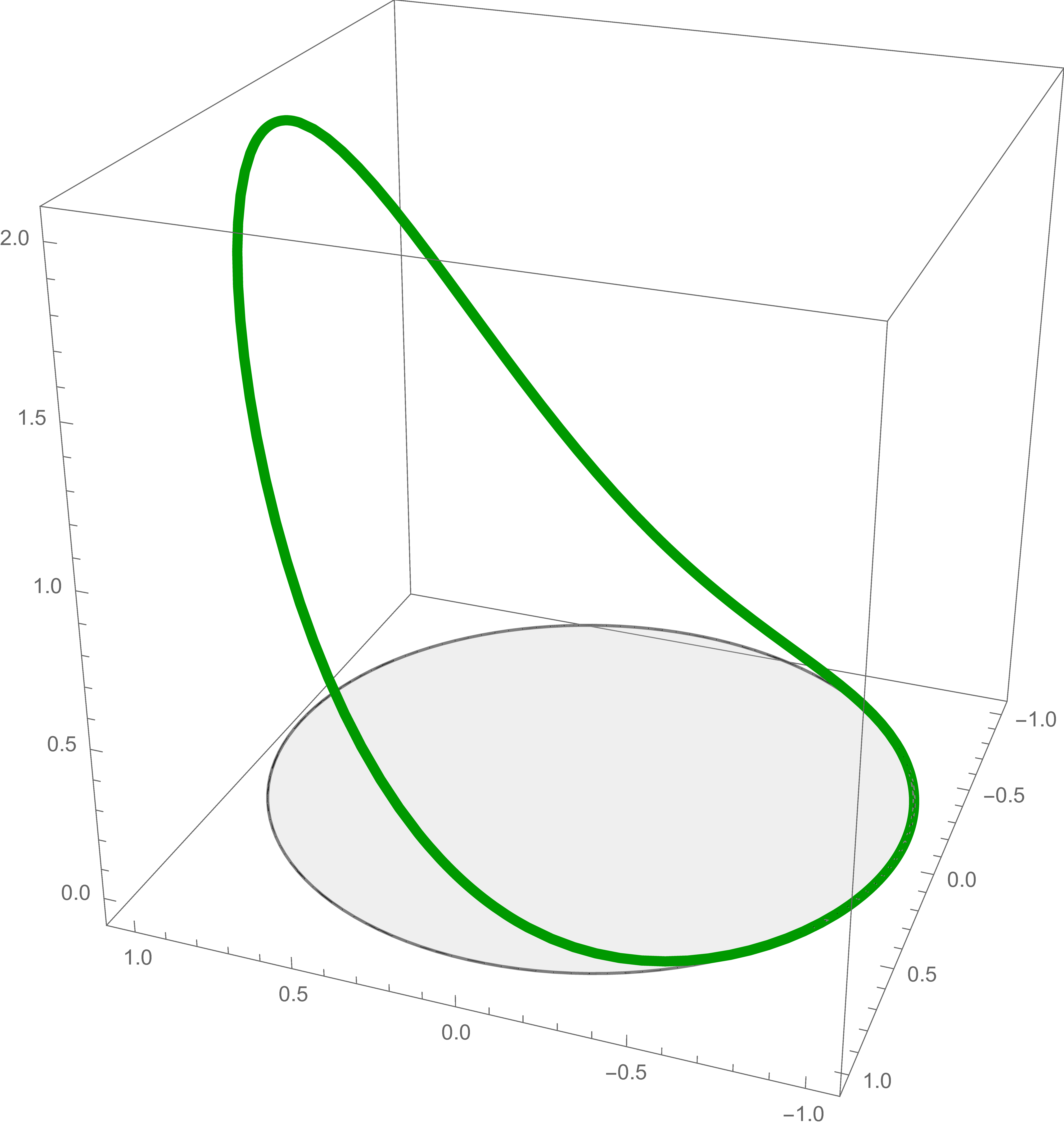
- Let \[ f(\theta) = 2 \bigl(\cos(\theta/2) \bigr)^6, \quad \theta \in [-\pi, \pi], \] in the boundary condition for Laplace's equation on a disk. Based on the last identity in the preceding item we have the following identity for the given boundary condition: \[ 2 \bigl(\cos(\theta/2) \bigr)^6 = \frac{5}{8}+\frac{15}{16} \cos (\theta ) +\frac{3}{8}\cos (2 \theta ) + \frac{1}{16} \cos (3 \theta ). \] From this formula we can read out the coefficients \[ a_0 = \frac{5}{8}, \quad a_1= \frac{15}{16}, \quad a_2 = \frac{3}{8}, \quad a_3 = \frac{1}{16}, \] and all other coefficients are zero. Surprisingly, from these trigonometric identities we can also deduce the following integrals \begin{align*} \frac{5}{8} & = \frac{1}{2\pi} \int_{-\pi}^{\pi} 2 \bigl(\cos(\theta/2) \bigr)^6 d \theta \\ \frac{15}{16} & = \frac{1}{\pi} \int_{-\pi}^{\pi} 2 \bigl(\cos(\theta/2) \bigr)^6 \cos(\theta) d \theta \\ \frac{3}{8} & = \frac{1}{\pi} \int_{-\pi}^{\pi} 2 \bigl(\cos(\theta/2) \bigr)^6 \cos(2 \theta) d \theta \\ \frac{1}{16} & = \frac{1}{\pi} \int_{-\pi}^{\pi} 2 \bigl(\cos(\theta/2) \bigr)^6 \cos(3 \theta) d \theta \end{align*}
-
Hence, the exact solution of the boundary value problem on the unit disk with this specific boundary condition is
\[
w(r,\theta) = \frac{5}{8}+\frac{15}{16} r \cos (\theta )
+\frac{3}{8} r^2 \cos (2 \theta ) + \frac{1}{16} r^3 \cos (3 \theta ).
\]
The Mathematica code for the left picture above:
MyOptionsD =
  Sequence[ImageResolution -> 600, Axes -> True,
   AxesLabel -> {None, None, None},
   AxesOrigin -> {Automatic, Automatic, Automatic}, Boxed -> True,
   DisplayFunction -> Identity, FaceGrids -> None,
   FaceGridsStyle -> Automatic, ImageSize -> 500,
   Lighting -> {{"Ambient", White}}, BoundaryStyle -> None,
   Method -> {"DefaultGraphicsInteraction" -> {"Version" -> 1.2`,
       "TrackMousePosition" -> {True, False},
       "Effects" -> {"Highlight" -> {"ratio" -> 2},
         "HighlightPoint" -> {"ratio" -> 2},
         "Droplines" -> {"freeformCursorMode" -> True,
           "placement" -> {"x" -> "All", "y" -> "None"}}}},
     "RotationControl" -> "Globe"},
   PlotRangePadding -> {Scaled[0.02`], Scaled[0.02`], Scaled[0.02`]},
   Ticks -> {Automatic, Automatic, Automatic},
   ViewPoint -> {-1.0311155006393165`, 2.874130096265292`,
     1.4581416303238175`},
   ViewVertical -> {0.15265090977010184`, -0.40303458278204485`,
     0.9023640201316004`}];
fbth[\[Theta]_] = 2 Cos[\[Theta]/2]^6;
gtfbth = ParametricPlot3D[{Cos[\[Theta]], Sin[\[Theta]],
    fbth[\[Theta]]}, {\[Theta], -Pi, Pi},
   PlotStyle -> {RGBColor[0, 0.6, 0], Thickness[0.01]},
   PlotPoints -> {100}];
disks = Graphics3D[
   {
    {FaceForm[RGBColor[0.75, 0.75, 0.75]], Opacity[0.25],
     Polygon[{Cos[#], Sin[#], 0} & /@
       Range[-Pi, Pi, Pi/64]]}, {GrayLevel[0.5], Thickness[0.003],
     Line[{Cos[#], Sin[#], 0} & /@ Range[-Pi, Pi, Pi/64]]}
    }, Lighting -> {{"Ambient", White}}
   ];
EqSolDiskBC =
 Show[{gtfbth, disks},
  PlotRange -> {{-1.05, 1.05}, {-1.05, 1.05}, {-.05, 2.05}},
  BoxRatios -> {1, 1, 1}, MyOptionsD]
The Mathematica code for the right picture above (it uses some definitions in the preceding command):Clear[wwSd]; wwSd[r_, \[Theta]_] := 5/8 + 15 /16 r Cos[\[Theta]] + 3/8 r^2 Cos[2 \[Theta]] + 1/16 r^3 Cos[3 \[Theta]]; soluD = ParametricPlot3D[{r Cos[\[Theta]], r Sin[\[Theta]], wwSd[r, \[Theta]]}, {r, 0, 1}, {\[Theta], -Pi, Pi}, PlotStyle -> {Opacity[0.7]}, PlotPoints -> {30, 100}, Mesh -> {10, 50}, MeshStyle -> {{Thickness[0.002], RGBColor[0, 0.5, 0.5], Opacity[0.5]}, {Thickness[0.002], RGBColor[0, 0.5, 0.5], Opacity[0.5]}}, BoundaryStyle -> Directive[{Thickness[0.002], RGBColor[0, 0.5, 0.5], Opacity[0.5]}]]; EqSolDisk = Show[{soluD, gtfbth, disks}, PlotRange -> {{-1.05, 1.05}, {-1.05, 1.05}, {-.05, 2.05}}, BoxRatios -> {1, 1, 1}, MyOptionsD]
- I updated the website dedicated to solving Laplace's equation on a rectangle by explanation of how we calculate the coefficients \(a_n\), \(b_n\), \(c_n\) and \(d_n\). In fact, I gave a detailed explanation for \(a_n\), and I hope that you can get the formulas for others by analogy, see Laplace's equation on a Rectangle. See also Section 2.5.1 in the textbook.
- I also update the notebook Equilibrium_temperature_2D_v12.nb with a detailed explanation of the method that we use to calculate \(a_n\), \(b_n\), \(c_n\) and \(d_n\). In this notebook, I show all the steps for each of the coefficients. You can check a pdf printout of this notebook at Equilibrium_temperature_2D_v12.pdf. You can download the notebook here Equilibrium_temperature_2D_v12.nb
- The most important formulas in this context are integrals of squares of trigonometric functions cosine and sine. The pictures below illustrate a "geometric" reason for the equalities that we derived in class: \[ \int_{-\pi}^{\pi} \bigl(\cos (k\mkern 1px x) \bigr)^2 dx = \pi \qquad \text{whenever} \qquad k \in \mathbb{N}. \] Similar pictures can be created on any interval $[-L, L]$ with $L \gt 0$. Those pictures would prove \[ \int_{-L}^{L} \biggl(\cos \Bigl( \frac{k\mkern 1px \pi}{L} x \Bigr) \biggr)^2 dx = L \qquad \text{whenever} \qquad k \in \mathbb{N}. \]
-
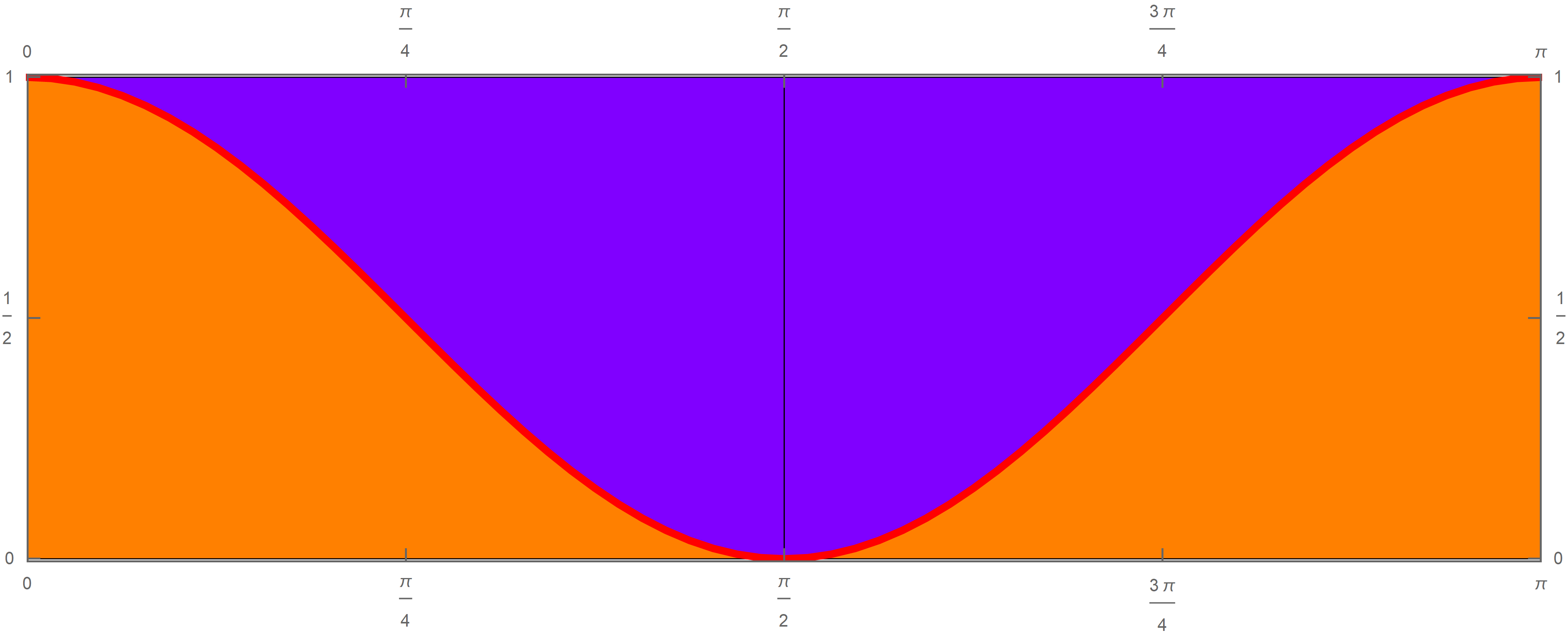
Below are pictures and animations that first justify the fact
\[
\int_{0i}^{\pi/2} \bigl(\cos x \bigr)^2 dx = \frac{\pi}{4}
\]
In fact, there are no integrals in these
visual and colorful proofs. These questions could be explored in any trigonometry class. For example, one could print colored pictures from below and ask students to use scissors to perform a proof. That is well known method of proofs: Scissors Method. -
A trigonometry question: Given that the equation of the red curve in the picture below is
\[
y = (\cos x)^2,
\]
calculate the orange area?
-
The following picture could be regarded as a hint. Or, you can print out the picture below hand it out to trigonometry students, and ask them to use scissors to do the calculation. Colors help.
-
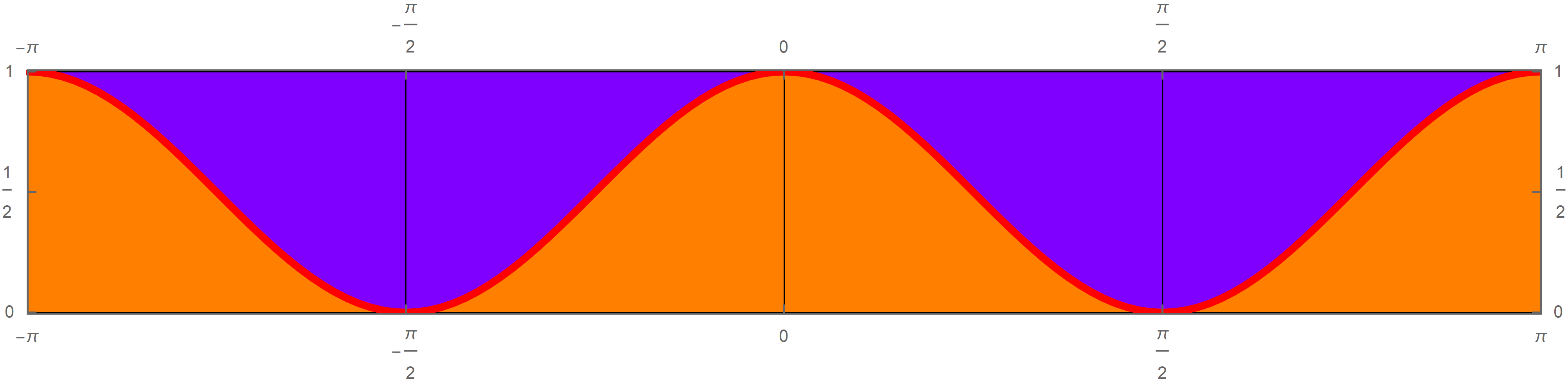
Another task for trigonometry students:
-
Animations, always helpful, hopefully.
-
Try larger domains.
- Today, we began exploration of solving Laplace's equation on a rectangle. I wrote a webpage Laplace's equation on a Rectangle with my approach to this problem. That is Section 2.5.1 in the textbook.
- The notebook Equilibrium_temperature_2D_v12.nb contains a Mathematica implementation of finding the solution of the Laplace equation on a rectangle. A pdf printout of this notebook is Equilibrium_temperature_2D_v12.pdf. You can download the notebook here Equilibrium_temperature_2D_v12.nb
- In the context of separation of variables in Laplace's equation and beyond, we often encounter trigonometric and hyperbolic functions. Below, I will provide a brief overview of relevant concepts.
-
Let $P$ and $Q$ be continuous real valued functions defined on $\mathbb{R}$. Let $Y_1 : \mathbb{R} \rightarrow \mathbb{R}$ and $Y_2: \mathbb{R} \rightarrow \mathbb{R}$ be linearly independent solutions of the homogeneous linear equation (HLE) \begin{equation*} Y^{\prime\prime}(x)+P(x) Y^{\prime}(x)+Q(x)Y(x)= 0, \ x \in \mathbb{R}. \end{equation*} Then all solutions of the HLE are given by the formula \[ Y(x) = c_1 Y_1(x) + c_2 Y_2(x), \ \ x \in \mathbb{R}, \] where $c_1$ and $c_2$ are arbitrary constants.
The solution \[ Y(x) = c_1 Y_1(x) + c_2 Y_2(x), \ \ x \in \mathbb{R}, \] is called the general solution of the HLE.
A pair of linearly independent solutions of the HLE is called a fundamental set of solutions of the HLE.
Below, we always have $x \in \mathbb{R}$.
-
Let us take a closer look at two fundamental trigonometric functions
\[
x \mapsto \cos(x) \quad \text{and} \quad x \mapsto \sin(x).
\]
- Their derivatives are \[ \bigl( \cos(x) \bigr)' = - \sin(x) \quad \text{and} \quad \bigl( \sin(x) \bigr)' = \cos(x), \] and their second derivatives are \[ \bigl( \cos(x) \bigr)'' = - \cos(x) \quad \text{and} \quad \bigl( \sin(x) \bigr)'' = -\sin(x). \]
-
Therefore, $\cos(x)$ and $\sin(x)$ satisfy the following linear homogeneous second-order differential equation with constant coefficients \[ Y''(x) + Y(x) = 0. \] Since the preceding differential equation is linear homogeneous equation, any linear combination of $\cos(x)$ and $\sin(x)$ is also a solution. In fact, all solutions of the preceding differential equation are given by the following expression \[ c_1 \cos(x) + c_2 \sin(x), \quad \text{where} \quad c_1, c_2 \in \mathbb{R}. \] The preceding expression is called the general solution of $Y''(x) + Y(x) = 0.$
-
There is something special about $\cos(x)$ and $\sin(x)$ that I must mention here. Look at the values of $\cos(x)$ and $\sin(x)$ and its derivatives at $0$: \[ \begin{array}{c} \Big.\bigl(\cos(x)\bigr)\Big|_{x=0} = 1 \\ \Big.\bigl(\cos(x)\bigr)'\Big|_{x=0} = 0 \end{array} \qquad \text{and} \qquad \begin{array}{c} \Big.\bigl(\sin(x)\bigr)\Big|_{x=0} = 0 \\ \Big.\bigl(\sin(x)\bigr)'\Big|_{x=0} = 1 \end{array} \]
- There are many interesting functions that hide in the general solution. For example, for arbitrary $a, b \in \mathbb{R}$ the functions \begin{align*} x & \mapsto b \cos(x - a), \\[4pt] x & \mapsto b \sin(x-a), \\[4pt] x & \mapsto b \cos(a - x), \\[4pt] x & \mapsto b \sin(a-x). \end{align*} solve the differential equation $Y''(x) + Y(x) = 0.$ To convince yourself that this is true, just find the second derivative by using rules for the derivative: \begin{align*} \bigl( b \cos(x - a)\bigr)' & = -b \sin(x - a) , \\ \bigl( b \cos(x - a)\bigr)'' & = -b \cos(x - a). \end{align*} Hence, \[ \bigl( b \cos(x - a)\bigr)'' + b \cos(x - a) = 0. \] Further, \begin{align*} \bigl( b \sin(x-a)\bigr)' & = b \cos(x-a), \\ \bigl( b \sin(x-a)\bigr)'' & = -b \sin(x-a). \end{align*} Hence \[ \bigl( b \sin(x-a)\bigr)' + b \sin(x-a) = 0. \] Further, \begin{align*} \bigl( b \cos(a - x) \bigr)' & = b \sin(a - x) \\ \bigl( b \cos(a - x) \bigr)'' &= -b \cos(a - x). \end{align*} Hence, \[ \bigl( b \cos(a - x) \bigr)'' + b \cos(a - x) = 0. \] Further, \begin{align*} \bigl( b \sin(a-x)\bigr)' & = - b \cos(a-x), \\ \bigl( b \sin(a-x)\bigr)'' & = - b \sin(a-x). \end{align*} Hence, \[ \bigl( b \sin(a-x)\bigr)' + b \sin(a-x) = 0. \]
-
In this item we introduce two fundamental hyperbolic functions. We start with the linear homogeneous second-order differential equation with constant coefficients
\[
Y''(x) - Y(x) = 0.
\]
Notice that this equation is just a slight variation on the differential equation $Y''(x) + Y(x) = 0$ which leads to the famous trigonometric functions $\cos(x)$ and $\sin(x)$.
- What is the general solution of \[ Y''(x) - Y(x) = 0? \] Consider the functions \[ x \mapsto e^x \quad \text{and} \quad x \mapsto e^{-x}, \] and their derivatives \[ \bigl(e^x\bigr)' = e^x \quad \text{and} \quad \bigl(e^{-x}\bigr)' = - e^{-x}, \] and \[ \bigl(e^x\bigr)'' = e^x \quad \text{and} \quad \bigl(e^{-x}\bigr)'' = e^{-x}. \] Therefore, the general solution of $Y''(x) - Y(x) = 0$ is \[ c_1 e^{x} + c_2 e^{-x}, \quad c_1, c_2 \in \mathbb{R}. \]
- There are two solutions in the general solution given in the preceding item that stand out. Those are \[ x \mapsto \frac{1}{2} e^x + \frac{1}{2} e^{-x} = \cosh(x) \quad \text{and} \quad x \mapsto \frac{1}{2} e^x - \frac{1}{2} e^{-x} = \sinh(x). \] The function $\cosh$ is called the hyperbolic cosine and the function $\cosh$ is called the hyperbolic sine. You can learn more about them at the Wikipedia page Hyperbolic Functions.
- To familiarize ourselves with these functions, we take their derivatives \[ \bigl(\cosh(x)\bigr)' = \sinh(x) \quad \text{and} \quad \bigl( \sinh(x) \bigr)' = \cosh(x), \] and \[ \bigl(\cosh(x)\bigr)'' = \cosh(x) \quad \text{and} \quad \bigl( \sinh(x) \bigr)'' = \sinh(x), \] So, they clearly solve $Y''(x) - Y(x)=0$. But, more importantly, they have special properties. Look at the values of $\cosh(x)$ and $\sinh(x)$ and its derivatives at $0$: \[ \begin{array}{c} \Big.\bigl(\cosh(x)\bigr)\Big|_{x=0} = 1 \\ \Big.\bigl(\cosh(x)\bigr)'\Big|_{x=0} = 0 \end{array} \qquad \text{and} \qquad \begin{array}{c} \Big.\bigl(\sinh(x)\bigr)\Big|_{x=0} = 0 \\ \Big.\bigl(\sinh(x)\bigr)'\Big|_{x=0} = 1 \end{array} \] Very convenient!
- The hyperbolic trigonometric functions $\cosh(x)$ and $\sinh(x)$ give us another way to write the general solution of $Y''(x) - Y(x) = 0$: \[ c_1 \cosh(x) + c_2 \sinh(x), \quad \text{where} \quad c_1, c_2 \in \mathbb{R}. \]
- There are many interesting functions that hide in the general solution given in the preceding item. For example, for arbitrary $a, b \in \mathbb{R}$ the functions \begin{align*} x & \mapsto b \cosh(x - a), \\ x & \mapsto b \sinh(x-a), \\ x & \mapsto b \cosh(a - x), \\ x & \mapsto b \sinh(a-x). \end{align*} solve the differential equation $Y''(x) - Y(x) = 0.$ To convince yourself that this is true, just find the second derivative by using the rules for derivative: \begin{align*} \bigl( b \cosh(x - a)\bigr)' & = b \sin(x - a) , \\ \bigl( b \cosh(x - a)\bigr)'' & = b \cosh(x - a). \end{align*} Hence, \[ \bigl( b \cosh(x - a)\bigr)'' - b \cosh(x - a) = 0. \] Further, \begin{align*} \bigl( b \sinh(x-a)\bigr)' & = b \cosh(x-a), \\ \bigl( b \sinh(x-a)\bigr)'' & = b \sinh(x-a). \end{align*} Hence, \[ \bigl( b \sinh(x-a)\bigr)'' - b \sinh(x-a) = 0. \] Further, \begin{align*} \bigl( b \cosh(a - x) \bigr)' & = - b \sinh(a - x), \\ \bigl( b \cosh(a - x) \bigr)'' & = b \cosh(a - x). \end{align*} Hence, \[ \bigl( b \cosh(a - x) \bigr)'' - b \cosh(a - x) = 0. \] Further, \begin{align*} \bigl( b \sinh(a-x)\bigr)' & = - b \cosh(a-x), \\ \bigl( b \sinh(a-x)\bigr)'' & = b \sinh(a-x). \end{align*} Hence, \[ \bigl( b \sinh(a-x)\bigr)'' - b \sinh(a-x) = 0. \]
-
I did not expect this to be that long. But, I find it to be a nice story. The story continues by considering the trigonometric functions with different frequencies. For $\mu \gt 0$ consider
\[
x \mapsto \cos(\mu x) \quad \text{and} \quad x \mapsto \sin(\mu x).
\]
- The derivatives of the trigonometric functions given above are \[ \bigl( \cos(\mu x) \bigr)' = - \mu \sin(\mu x) \quad \text{and} \quad \bigl( \sin(\mu x) \bigr)' = \mu \cos(\mu x), \] and their second derivatives are \[ \bigl( \cos(\mu x) \bigr)'' = - \mu^2 \cos(\mu x) \quad \text{and} \quad \bigl( \sin(\mu x) \bigr)'' = -\mu^2 \sin(\mu x). \]
-
Therefore, $\cos(\mu x)$ and $\sin(\mu x)$ satisfy the following linear homogeneous second-order differential equation with constant coefficients \[ Y''(x) + \mu^2 Y(x) = 0. \] This equation can be written as an "eigenvalue equation" \[ -Y''(x) = \mu^2 Y(x) \] Since the preceding differential equation is linear homogeneous equation, any linear combination of $\cos(\mu x)$ and $\sin(\mu x)$ is also a solution. In fact, all solutions of the preceding differential equation are given by the following expression \[ c_1 \cos(\mu x) + c_2 \sin(\mu x), \quad \text{where} \quad c_1, c_2 \in \mathbb{R}. \] The preceding expression is called the general solution of $-Y''(x) = \mu^2 Y(x).$
- There are many interesting functions that hide in the general solution given in the preceding item. For example, for arbitrary $a, b \in \mathbb{R}$ the functions \begin{align*} x & \mapsto b \cos\bigl(\mu (x - a) \bigr), \\ x & \mapsto b \sin\bigl(\mu (x - a) \bigr), \\ x & \mapsto b \cos\bigl(\mu (a - x) \bigr), \\ x & \mapsto b \sin\bigl(\mu (a - x) \bigr), \end{align*} solve the differential equation $-Y''(x) = \mu^2 Y(x).$ To convince yourself that this is true, just find the second derivative by using the chain rule: \begin{align*} \bigl( b \cos\bigl(\mu (x - a) \bigr)\bigr)' & = - \mu b \sin\bigl(\mu (x - a) \bigr) , \\ \bigl( b \cos\bigl(\mu (x - a) \bigr)\bigr)'' & = - \mu^2 b \cos\bigl(\mu (x - a) \bigr). \end{align*} Hence, \[ \bigl( b \cos\bigl(\mu (x - a) \bigr)\bigr)'' + \mu^2 b \cos\bigl(\mu (x - a) \bigr) = 0. \] Further, \begin{align*} \bigl( b \sin\bigl(\mu (x - a) \bigr)\bigr)' & = \mu b \cos\bigl(\mu (x - a) \bigr), \\ \bigl( b \sin\bigl(\mu (x - a) \bigr)\bigr)'' &= -\mu^2 b \sin\bigl(\mu (x - a) \bigr). \end{align*} Hence, \[ \bigl( b \sin\bigl(\mu (x - a) \bigr)\bigr)'' + \mu^2 b \sin\bigl(\mu (x - a) \bigr) = 0. \] Further, \begin{align*} \bigl( b \cos\bigl(\mu (a - x) \bigr) \bigr) &= \mu b \sin\bigl(\mu (a - x) \bigr), \\ \bigl( b \cos\bigl(\mu (a - x) \bigr) \bigr)'' &= -\mu^2 b \cos\bigl(\mu (a - x) \bigr). \end{align*} Hence, \[ \bigl( b \cos\bigl(\mu (a - x) \bigr) \bigr)'' + \mu^2 b \cos\bigl(\mu (a - x) \bigr) = 0. \] Further, \begin{align*} \bigl( b \sin\bigl(\mu (a - x) \bigr) \bigr)' & = \mu b \sin\bigl(\mu (a - x) \bigr), \\ \bigl( b \sin\bigl(\mu (a - x) \bigr)\bigr)'' & = -\mu^2 b \sin\bigl(\mu (a - x) \bigr). \end{align*} Hence, \[ \bigl( b \sin\bigl(\mu (a - x) \bigr)\bigr)'' + \mu^2 b \sin\bigl(\mu (a - x) \bigr) = 0. \]
-
The story continues by considering the hyperbolic functions with scaled independent variable. For $\mu \gt 0$ consider
\[
x \mapsto \cosh(\mu x) \quad \text{and} \quad x \mapsto \sinh(\mu x).
\]
- The derivatives of the hyperbolic functions given above are \[ \bigl( \cosh(\mu x) \bigr)' = \mu \sinh(\mu x) \quad \text{and} \quad \bigl( \sinh(\mu x) \bigr)' = \mu \cosh(\mu x), \] and their second derivatives are \[ \bigl( \cosh(\mu x) \bigr)'' = \mu^2 \cosh(\mu x) \quad \text{and} \quad \bigl( \sinh(\mu x) \bigr)'' = \mu^2 \sinh(\mu x). \]
-
Therefore, $\cosh(\mu x)$ and $\sinh(\mu x)$ satisfy the following linear homogeneous second-order differential equation with constant coefficients \[ Y''(x) - \mu^2 Y(x) = 0. \] This equation can be written as an "eigenvalue equation" \[ Y''(x) = \mu^2 Y(x) \] Since the preceding differential equation is linear homogeneous equation, any linear combination of $\cosh(\mu x)$ and $\sinh(\mu x)$ is also a solution. In fact, all solutions of the preceding differential equation are given by the following expression \[ c_1 \cosh(\mu x) + c_2 \sinh(\mu x), \quad \text{where} \quad c_1, c_2 \in \mathbb{R}. \] The preceding expression is called the general solution of $Y''(x) = \mu^2 Y(x).$
- There are many interesting functions that hide in the general solution given in the preceding item. For example, for arbitrary $a, b \in \mathbb{R}$ the functions \begin{align*} x & \mapsto b \cosh\bigl(\mu (x - a) \bigr), \\ x & \mapsto b \sinh\bigl(\mu (x - a) \bigr), \\ x & \mapsto b \cosh\bigl(\mu (a - x) \bigr), \\ x & \mapsto b \sinh\bigl(\mu (a - x) \bigr), \end{align*} solve the differential equation $Y''(x) = \mu^2 Y(x).$ To convince yourself that this is true, just find the second derivative by using the chain rule: \begin{align*} \bigl( b \cosh\bigl(\mu (x - a) \bigr)\bigr)' & = \mu b \sinh\bigl(\mu (x - a) \bigr) , \\ \bigl( b \cosh\bigl(\mu (x - a) \bigr)\bigr)'' & = \mu^2 b \cosh\bigl(\mu (x - a) \bigr). \end{align*} Hence, \[ \bigl( b \cosh\bigl(\mu (x - a) \bigr)\bigr)'' - \mu^2 b \cosh\bigl(\mu (x - a) \bigr) = 0. \] Further, \begin{align*} \bigl( b \sinh\bigl(\mu (x - a) \bigr)\bigr)' &= \mu b \cosh\bigl(\mu (x - a) \bigr), \\ \bigl( b \sinh\bigl(\mu (x - a) \bigr)\bigr)'' & = \mu^2 b \sinh\bigl(\mu (x - a) \bigr). \end{align*} Hence, \[ \bigl( b \sinh\bigl(\mu (x - a) \bigr)\bigr)'' - \mu^2 b \sinh\bigl(\mu (x - a) \bigr) = 0. \] Further, \begin{align*} \bigl( b \cosh\bigl(\mu (a - x) \bigr) \bigr)' & = -\mu b \sinh\bigl(\mu (a - x) \bigr),\\ \bigl( b \cosh\bigl(\mu (a - x) \bigr) \bigr)'' & = \mu^2 b \cosh\bigl(\mu (a - x) \bigr). \end{align*} Hence, \[ \bigl( b \cosh\bigl(\mu (a - x) \bigr) \bigr)'' - \mu^2 b \cosh\bigl(\mu (a - x) \bigr) = 0. \] Further, \begin{align*} \bigl( b \sinh\bigl(\mu (a - x) \bigr)\bigr)' & = - \mu b \cosh\bigl(\mu (a - x) \bigr), \\ \bigl( b \sinh\bigl(\mu (a - x) \bigr)\bigr)'' &= \mu^2 b \sinh\bigl(\mu (a - x) \bigr). \end{align*} Hence, \[ \bigl( b \sinh\bigl(\mu (a - x) \bigr)\bigr)'' - \mu^2 b \sinh\bigl(\mu (a - x) \bigr) = 0. \]
- This week we are discussing Fourier's Method of Separation of Variables. The relevant sections of the textbook is 2.3.1, 2.3.2, 2.3.3, 2.3.4. Below is a short story of this method.
- Start. We ignore the initial conditions and consider the Partial Differential Equation and the Boundary Conditions. Please have in mind that we can consider a variety of Boundary Conditions. Below are the Dirichlet Boundary Conditions. We can consider insulated endpoints (those are Neuman Boundary Conditions), and more. \[ \require{bbox} \bbox[5px,border:4px solid orange]{ \begin{alignedat}{3} & \text{PDE:} \qquad & & \frac{\partial \color{#FF0000}{u}}{\partial t}(x,t) = \color{#009900}{\varkappa} \frac{\partial^2 \color{#FF0000}{u}}{\partial x^2}(x,t), \qquad && x \in [0, \color{#009900}{L}], \quad t \geq 0, \\[5pt] & \text{BCs:} \qquad & & \color{#FF0000}{u}(0,t) = 0, \quad \color{#FF0000}{u}(\color{#009900}{L},t) = 0, \qquad && t \geq 0. \end{alignedat} } \]
- Fourier's Brilliant Idea. We expect that the orange box problem has many solutions. So, we hope that it has solutions that are products like in the light-blue box: \[ \bbox[5px,border:4px solid #8888FF]{ \color{#FF0000}{u}(x,t) = \color{#FF0000}{A}(x) \color{#FF0000}{B}(t) } \] One guiding principle in Mathematics is to try to reduce a complicated problem to simpler ones. Functions with two variables are more complicated than functions of a single variable. Thus, what is stated in the light-blue box replaces red function of two variables with TWO red functions of a single variables. It turns out, this is a reduction in complexity.
- Some algebra is skipped here. Please recover that algebra on your own, look at the textbook. If still unclear, post in Canvas Discussion.
- Substitute \(\color{#FF0000}{u}(x,t) = \color{#FF0000}{A}(x) \color{#FF0000}{B}(t)\) in the orange box to get \[ \require{bbox} \bbox[5px,border:4px solid orange]{ \begin{alignedat}{3} & \text{ODEs:} \qquad & & \frac{\color{#FF0000}{B}'(t)}{\color{#009900}{\varkappa} \color{#FF0000}{B}(t)} = \frac{\color{#FF0000}{A}''(x)}{\color{#FF0000}{A}(x)} = - \color{#FF0000}{\lambda}, \qquad && x \in [0, \color{#009900}{L}], \quad t \geq 0, \\[5pt] & \text{BCs:} \qquad & & \color{#FF0000}{A}(0) = 0, \quad \color{#FF0000}{A}(\color{#009900}{L}) = 0. \qquad && \end{alignedat} } \]
- And finally and beautifully we get two separate Ordinary Differential Equations problems. The first Ordinary Differential Equation is an equation in time, the second Ordinary Differential Equation is an eigenvalue problem involving boundary values, such problems are called Boundary Eigenvalue Problems (BEP). \[ \require{bbox} \text{time ODE:} \quad \bbox[5px,border:4px solid orange]{ \color{#FF0000}{B}'(t) = - \color{#FF0000}{\lambda} \color{#009900}{\varkappa}\mkern 2mu \color{#FF0000}{B}(t), \quad t \geq 0, } \] \[ \require{bbox} \text{space BEP:} \quad \bbox[5px,border:4px solid orange]{ \begin{alignedat}{3} & \text{ODE:} \qquad & & - \color{#FF0000}{A}''(x) = \color{#FF0000}{\lambda}\mkern 1mu \color{#FF0000}{A}(x), \quad && x \in [0, \color{#009900}{L}], \\[5pt] & \text{BCs:} \quad & & \color{#FF0000}{A}(0) = 0, \quad \color{#FF0000}{A}(\color{#009900}{L}) = 0. \qquad && \end{alignedat} } \]
- We can solve the ODE in the first orange box: \[ B(t) = \exp\bigl( - \color{#FF0000}{\lambda} \color{#009900}{\varkappa}\mkern 2mu t \bigr), \quad t \geq 0. \] Admittedly, \(B(t)\) is not completely green yet, but, the red function \(\color{#FF0000}{B}(t)\) has been replaced by the red real number \(\color{#FF0000}{\lambda}\) which we stand chance of obtaining from the second orange box.
-
Let us analyse the second orange box. The Ordinary Differential Equation will become a little friendlier if we replace \(\color{#FF0000}{\lambda} = \color{#FF0000}{\mu}^2\) with \(\mu \geq 0\), and write
\[
\require{bbox}
\bbox[5px,border:4px solid orange]{
\text{ODE:} \qquad
\color{#FF0000}{A}''(x) + \color{#FF0000}{\mu}^2\mkern 0mu \color{#FF0000}{A}(x) = 0, \quad x \in [0, \color{#009900}{L}].
}
\]
This equation is a second order linear homogeneous equation that you studied in an Ordinary Differential Equations class. In fact this is, so called mass-spring equation, see Wikipedia's page Simple Harmonic Motion and the snippet below.
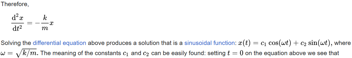
Thus, the general solution of the second-order linear homogeneous equation in the last orange box is \[ A(x) = \color{#FF0000}{c_1} \cos(\color{#FF0000}{\mu}\mkern 1mu x) + \color{#FF0000}{c_2} \sin(\color{#FF0000}{\mu}\mkern 1mu x). \] The remarkable feature of the above equation for \(A(x)\) is that the redness of \(A(x)\) has been replaced by the redness of the coefficients \(\color{#FF0000}{c_1}\) and \(\color{#FF0000}{c_2}\) and the redness of \(\color{#FF0000}{\mu}\); all being real numbers, this is much better than seeking an unknown function.
-
To determine \(\color{#FF0000}{c_1}\) and \(\color{#FF0000}{c_2}\) and the redness of \(\color{#FF0000}{\mu}\), we recall the Boundary Conditions:
\[
\require{bbox}
\bbox[5px,border:4px solid orange]{
\text{BCs:} \qquad \color{#FF0000}{A}(0) = 0, \quad \color{#FF0000}{A}(\color{#009900}{L}) = 0.
}
\]
and recall that we are looking for a nonzero functions
\[
A(x) =
\color{#FF0000}{c_1} \cos(\color{#FF0000}{\mu}\mkern 1mu x)
+ \color{#FF0000}{c_2} \sin(\color{#FF0000}{\mu}\mkern 1mu x)
\]
which satisfy the above boundary conditions.
- Substituting \(x=0\) and \(x = \color{#009900}{L}\) in the general solution for \(A(x)\) we get the system of equations: \begin{align*} \color{#FF0000}{c_1} \cos(\color{#FF0000}{\mu}\mkern 1mu 0) + \color{#FF0000}{c_2} \sin(\color{#FF0000}{\mu}\mkern 1mu 0) & = 0 \\ \color{#FF0000}{c_1} \cos(\color{#FF0000}{\mu}\mkern 1mu \color{#009900}{L}) + \color{#FF0000}{c_2} \sin(\color{#FF0000}{\mu}\mkern 1mu \color{#009900}{L}) & = 0 \\ \end{align*} I know, one can solve this system for \(\color{#FF0000}{c_1}\) and \(\color{#FF0000}{c_2}\) by elimination. But, I will solve it in a way that is applicable to more complicated settings that we will encounter later in the quarter.
- I rewrite the above system in matrix form: \[ \begin{bmatrix} 1 & 0 \\ \cos(\color{#FF0000}{\mu}\mkern 1mu \color{#009900}{L}) & \sin(\color{#FF0000}{\mu}\mkern 1mu \color{#009900}{L}) \end{bmatrix} \begin{bmatrix} \color{#FF0000}{c_1} \\ \color{#FF0000}{c_2} \end{bmatrix} = \begin{bmatrix} 0 \\ 0 \end{bmatrix}. \] First, I see that this is a homogeneous matrix equation; second I recall that we seek a nontrivial solution $\begin{bmatrix} \color{#FF0000}{c_1} \\ \color{#FF0000}{c_2} \end{bmatrix} \neq \begin{bmatrix} 0 \\ 0 \end{bmatrix}$. Recall that a homogeneous matrix equation has a nontrivial solution if and only if \[ \det \begin{bmatrix} 1 & 0 \\ \cos(\color{#FF0000}{\mu}\mkern 1mu \color{#009900}{L}) & \sin(\color{#FF0000}{\mu}\mkern 1mu \color{#009900}{L}) \end{bmatrix} = 0. \] Since, \[ \det \begin{bmatrix} 1 & 0 \\ \cos(\color{#FF0000}{\mu}\mkern 1mu \color{#009900}{L}) & \sin(\color{#FF0000}{\mu}\mkern 1mu \color{#009900}{L}) \end{bmatrix} = \sin(\color{#FF0000}{\mu}\mkern 1mu \color{#009900}{L}), \] the above matrix equation has a nontrivial solution if and only if \[ \sin(\color{#FF0000}{\mu}\mkern 1mu \color{#009900}{L}) = 0. \] Since we assume \(\color{#FF0000}{\mu} \geq 0\), we have solutions for \(\color{#FF0000}{\mu}\): \[ \color{#FF0000}{\mu} = \frac{k \mkern 1mu \pi}{\color{#009900}{L}}, \quad \text{where} \quad k \in \mathbb{N} = \{1,2,3,\ldots\}. \] With such \(\mu\)-s we have the nontrivial solution for \(\color{#FF0000}{c_1}\) and \(\color{#FF0000}{c_2}\): \[ \begin{bmatrix} \color{#FF0000}{c_1} \\ \color{#FF0000}{c_2} \end{bmatrix} = {c_2} \begin{bmatrix} 0 \\ 1 \end{bmatrix}, \] where \(c_2\) is a nonzero real number. As we did before we can take \(c_2 = 1\) and \(c_1 = 0\). Thus the corresponding nonzero function \(A(x)\) is \[ A_k(x) = \sin\Bigl(\frac{k \mkern 1mu \pi}{\color{#009900}{L}} \mkern 1mu x \Bigr), \quad \text{where} \quad k \in \mathbb{N}. \]
- Finally with the \({\mu}\) that we calculated we can calculate \(\color{#FF0000}{\lambda}\): \[ \color{#FF0000}{\lambda} = \mu^2 = \frac{k^2 \mkern 1mu \pi^2}{\color{#009900}{L^2}}, \quad \text{where} \quad k \in \mathbb{N}. \] And with \({\lambda}\) we can calculate the corresponding function \(B(t)\): \[ B_k(t) = \exp\Bigl( - \frac{k^2 \mkern 1mu \pi^2}{\color{#009900}{L^2}} \color{#009900}{\varkappa}\mkern 2mu t \Bigr),\quad \text{where} \quad k \in \mathbb{N}. \]
- Putting everything together, we have a sequence of solutins \[ u_k(x,t) = \sin\Bigl(\frac{k \mkern 1mu \pi}{\color{#009900}{L}} \mkern 1mu x \Bigr) \exp\Bigl( - \frac{k^2 \mkern 1mu \pi^2}{\color{#009900}{L^2}} \color{#009900}{\varkappa}\mkern 2mu t \Bigr),\quad \text{where} \quad k \in \mathbb{N}. \]
- Finally, using the sequence of solutions found in the preceding item, the linear combinations of the members of this sequence, even infinite ones are also solutions. For, now we can consider only finite sums: \[ u(x,t) = \sum_{k=1}^{n} c_k \sin\Bigl(\mkern -1mu\frac{k \mkern 1mu \pi}{\color{#009900}{L}} \mkern 1mu x\mkern -1mu\Bigr) \exp\Bigl(\mkern -2mu -\frac{k^2 \mkern 1mu \pi^2}{\color{#009900}{L^2}} \color{#009900}{\varkappa}\mkern 2mu t \mkern -1mu\Bigr), \] where \(n\) is a large positive integer and \(c_1,\ldots,c_n\) are arbitrary real numbers.
- Today we discussed Fourier's Method of Separation of Variables. The relevant sections of the textbook is 2.3.1, 2.3.2, 2.3.3, 2.3.4.
- We will use Fourier’s Method of Separation of Variables in various forms throughout the rest of the quarter, so it is essential to grasp its elegance and intricacies as soon as possible.
- We considered the homogeneous heat equation in a one-dimensional rod of length $L$ subject to the Dirichlet boundary conditions: \[ \frac{\partial u}{\partial t}(x,t) = \kappa \frac{\partial^2 u}{\partial x^2}(x,t) \qquad x \in [0,L], \quad t \geq 0, \] subject to the Boundary Conditions: \[ u(0,t) = 0 \quad \text{and} \quad u(L,t) = 0 \quad \text{for all} \quad t \geq 0. \] Notice that in the heat equation $\frac{\partial u}{\partial t} = \kappa \frac{\partial^2 u}{\partial x^2}$ I write $\kappa$, the Greek lower case letter kappa, instead of $k$ in the book. This constant is called thermal diffusivity. It is a complicated constant given by \[ \kappa = \frac{K_0}{c \, \rho}, \] where $K_0$ is the thermal conductivity constant from Fourier's Law, $c$ is the specific heat and $\rho$ is the mass density of the material. I do not like $k$ since $k$ is commonly used as a counting index in series, and we will be using infinite series all the time in the rest of the quarter.
- The brilliant idea to find solutions of the problem stated in the preceding item is to look for a solution in which the independent variables are separated in two functions $A$ and $B$: \[ u(x,t) = A(x) \mkern 1mu B(t). \] The brilliancy of the above idea is that one unpleasant unknown function $u(x,t)$ of two independent variables is replaced by two unknown functions $A(x)$ and $B(t)$, but each one of which is a function of a single independent variable. There is no guarantee that this idea will work. But, it is brilliant and amazing since it works, as we will see later.
-
Although we did not finish the process until the end, I will state the final solutions for $A(x)$ and $B(t)$: \begin{align*} B(t) & = \exp\mkern-4mu\left(\!-\frac{m^2 \pi^2}{L^2} \kappa\, t \right), \\ A(x) & = \sin\mkern-4mu\left(\frac{m \pi}{L} x\right), \end{align*} where $\kappa$ and $L$ are given positive real numbers and $m$ is any positive integer.
Thus, we have obtained the sequence of solutions for $u(x,t)$ given by \[ u(x,t) = \exp\mkern-4mu\left(\!-\frac{m^2 \pi^2}{L^2} \kappa\, t \right) \sin\mkern-4mu\left(\frac{m \pi}{L} x\right) \quad \text{where} \quad m \in \mathbb{N}. \] We use $\mathbb{N}$ to denote the set of all positive integers. A good exercise is to verify that the preceding formula for $u(x,t)$ indeed solves the heat equation with the Dirichlet boundary conditions, the problem stated above.
- Today, in a Zoom class, I presented my version of Section 1.5: Derivation of the Heat Equation in Two or Three Dimensions. This derivation uses concepts introduced in Math 225, the second quarter of Multivariable Calculus. However, by connecting the content to integral calculus in one variable, I hope I made it understandable.
- Due to Monday and Tuesday's class cancellations, I have written down the key content we planned to discuss here and on the linked page.
-
The webpage The Laplacian in Polar Coordinates contains a derivation of the Laplacian in polar coordinates: \[ \bigl(\nabla^2 w \bigr) (r,\theta) = \frac{1}{r^2} \frac{\partial^2 w}{\partial \theta^2}(r,\theta) + \frac{1}{r} \frac{\partial}{\partial r} \left( r \frac{\partial w}{\partial r}(r,\theta) \right). \] Here $w(r,\theta)$ is a function of $r \in (0,+\infty)$ and $\theta \in [0, 2\pi)$.
-
For example, consider the following function in the orthogonal coordinate system $xy$, \[ u(x,y) = x y\bigl(x^2 + y^2\bigr), \quad x,y \in \mathbb{R}. \] One can think of this function as giving a temperature at each point in the $xy$-plane. So, at the point $P$ whose coordinates in $xy$ orthogonal coordinate system are $(2,2)$ the temperature is $32.$ The same temperature in polar coordinates is given by the function \[ w(r,\theta) = r^4 (\cos \theta)(\sin \theta), \quad r \in [0,+\infty), \quad \theta \in [0, 2 \pi). \] The same point $P$ from above has coordinates $r = 2\sqrt{2},$ $\theta = \pi/4.$ So, the temperature at the point $P$ is \[ w\bigl(2\sqrt{2}, \pi/4 \bigr) = 2^4 2^2 (\sqrt{2}/2) (\sqrt{2}/2) = 32. \] The Laplacian of the function $u(x,y)$ is \[ (\nabla^2 u)(x,y) = \frac{\partial^2 u}{\partial x^2}(x,y) + \frac{\partial^2 u}{\partial y^2}(x,y) = 12 x y. \] The Laplacian of the function $w(r,\theta)$ is \[ (\nabla^2 w)(r,\theta) = \frac{1}{r^2} \frac{\partial^2 w}{\partial \theta^2}(r,\theta) + \frac{1}{r} \frac{\partial}{\partial r} \left( r \frac{\partial w}{\partial r}(r,\theta) \right) = 12 r^2 (\cos \theta)(\sin \theta). \] As expected, we have \[ 12xy \quad \text{in polar coordinates is} \quad 12 r^2 (\cos \theta)(\sin \theta). \]
- The Laplacian in spherical coordinates: \[ \Delta w = \nabla^2 w = {1 \over \rho^2} {\frac{\partial}{\partial \rho}} \left(\rho^2 {\frac{\partial w}{\partial \rho}} \right) + {\frac{1}{\rho^2 \sin \theta}} {\frac{\partial}{\partial \theta}} \left( (\sin \theta) {\frac{\partial w}{\partial \theta}} \right) + {1 \over \rho^2 (\sin \theta)^2} {\partial^2 w \over \partial \phi^2}. \] Here $w(\theta,\phi,\rho)$ is a function of $\rho \in (0,+\infty)$, $\theta \in [0, 2\pi),$ and $\phi \in [0,\pi]$.
-
Three related problems:
-
Problem 1.
Assume that the temperature is circularly symmetric: \( w = w(r,t) \), where \( r^2 = x^2 + y^2 \).
We will derive the heat equation for this problem. Consider any circular annulus \( a \leq r \leq b \).
- Show that the total heat energy is \( 2\pi c \rho \int_{a}^{b} w(r,t) \, dr \).
- Show that the flow of heat energy per unit time out of the annulus at \( r = b \) is \[ -2\pi b K_0 \frac{\partial w}{\partial r}(b,t). \] A similar result holds at \( r = a \).
- Use the preceding two parts to derive the circularly symmetric heat equation without sources: \[ \frac{\partial w}{\partial t}(r,t) = \frac{k}{r} \frac{\partial}{\partial r} \left( r \frac{\partial w}{\partial r}(r,t) \right). \]
- Problem 2. Let $a$ and $b$ be real numbers such that $a \lt b$. Determine the equilibrium temperature distribution inside a circular annulus \[ \bigl\{(r,\theta) \in (0,+\infty)\times[0,2\pi) : a \leq r \leq b \bigr\} \] if the outer radius is insulated and the inner radius is kept at the constant temperature $T_a$. Assume that all other relevant physical constants are equal to $1$.
-
Problem 3.
Consider the heat equation for a uniform annulus between the two concentric circles, both circles are centered at the origin. The inner circle has the radius $1$ and the outer circle has the radius $b$ with $b \gt 1$. All other relevant physical constants are equal to $1$. We assume that the temperature $w(r,t)$ is circularly symmetric (that is the temperature is constant along the circles centered at the origin). The heat equation in this case is
\begin{align*}
\frac{\partial w}{\partial t}(r,t) = \frac{1}{r} \frac{\partial}{\partial r} \left( r \frac{\partial w}{\partial r}(r,t) \right)& + r \\
\text{subject to} & \quad \frac{\partial w}{\partial r}(1,t)=5, \quad\frac{\partial w}{\partial r}(b,t)=-4.
\end{align*}
Notice that there are internal sources $Q(r) = r$ of thermal energy present in the annulus.
- For what value of $b \gt 1$ the given partial differential equation with the boundary conditions has an equilibrium temperature distribution?
- What is the heat energy generated per second in the annulus by the internal sources of heat energy? Use this result and the boundary conditions to support your answer in i.
- Suppose that the initial temperature distribution is $w(r,0) = f(r)$. Find the total thermal energy in the rod as a function of time. Use the answer obtained here to support your answer in i.
- Solution. Part i. An equilibrium solution of the given partial differential equation must satisfy \[ \frac{1}{r} \frac{\partial}{\partial r} \left( r \frac{\partial w}{\partial r}(r,t) \right) + r = 0. \] Solving this equation using the methods of integral calculus we obtain \[ w(r) = -\frac{1}{9} r^3 + c_1 \ln(r) + c_2. \] Next we need to determine the constants $c_1$ and $c_2$ such that \[ \frac{\partial w}{\partial r}(1)=5, \quad\frac{\partial w}{\partial r}(b)=-4. \] Thus we need to solve \[ -\frac{1}{3} 1^2 + c_1 \frac{1}{1} = 5, \quad -\frac{1}{3} b^2 + c_1 \frac{1}{b} = -4. \] Thus, $c_1 = 16/3,$ and $b$ must satisfy \[ -\frac{1}{3} b^2 + \frac{16}{3b} = -4, \] that is \[ b^3 - 12 b -16 = 0. \] Since \[ b^3 - 12 b -16 =(b-4)(b+2)(b+2), \] we deduce that for $b=4$, the given problem has an equilibrium solution.
-
Part ii. The internal sources in the annulus are given by $Q(r) = r$ where $1 \leq r \leq b$. The units of this function are $\displaystyle \frac{\operatorname{cal}}{\operatorname{cm}^3 \operatorname{sec}}.$ To get the total heat energy generated we need to integrate the function $Q(r)$ over the annulus. Since the height of the annulus is $1$, the total heat energy generated in the annulus is \[ \int_{0}^{2\pi} \int_1^b r \mkern 1mu r \mkern 1mu dr \mkern 1mu d\theta = \frac{2}{3}\bigl(b^3 - 1\bigr)\mkern 1mu \pi. \]
The given boundary conditions tell us about the heat energy that leaves the annulus. Based on Fourier's Law the flux along the inner circle is $-5$ in units $\frac{\operatorname{cal}}{\operatorname{cm}^2 \operatorname{sec}}.$ To get the total heat that leaves the annulus along the inner circle we multiply $5$ with the surface area $2\pi$, getting $10\pi$. The flux along the outer circle is $4$ in units $\frac{\operatorname{cal}}{\operatorname{cm}^2 \operatorname{sec}}.$ To get the total heat that leaves the annulus along the outer circle we multiply $4$ with the surface area $2b\pi$, getting $8 b \pi$. Thus the total amount of the heat energy that leaves the annulus is $10\pi+8 b \pi$.
For the annulus to have the equilibrium temperature we must have the heat energy generated in the annulus equal to the heat energy leaving the annulus. That is: \[ \frac{2}{3}\bigl(b^3 - 1\bigr)\mkern 1mu \pi = 10\pi+8 b \pi. \] The last equation simplifies to \[ b^3 - 12 b - 16 = 0, \] the same equation we obtained in i.
- Part iii. This part is a little tricky. It follows the reasoning presented in the derivation of the heat equation. Denote by $E(t)$ the amount of the heat energy in the annulus at time $t$. By the definition of the heat energy it depends on the temperature, the mass density and the specific heat. Since in this problem the mass density and the specific heat are both equal to $1$, the heat energy of the annulus is \begin{align*} E(t) & = \int_0^{2\pi} \int_0^b w(r,t)\mkern 1mu r \mkern 1mu dr d\theta \\ & = 2\pi \int_0^b w(r,t)\mkern 1mu r \mkern 1mu dr, \end{align*} with the initial condition \begin{align*} E(0) & = \int_0^{2\pi} \int_0^b f(r)\mkern 1mu r \mkern 1mu dr d\theta \\ &= 2 \pi \int_0^b f(r)\mkern 1mu r \mkern 1mu dr. \end{align*} The above formula for $E(t)$ is not very useful, but, we can differentiate with respect to $t$ and get \begin{align*} E'(t) & = \frac{d}{dt} 2\pi \int_0^b w(r,t)\mkern 1mu r \mkern 1mu dr \\ & = 2\pi \int_0^b \frac{\partial w}{\partial t}(r,t)\mkern 1mu r \mkern 1mu dr \end{align*} Now we recall the given equation \begin{equation*} \frac{\partial w}{\partial t}(r,t) = \frac{1}{r} \frac{\partial}{\partial r} \left( r \frac{\partial w}{\partial r}(r,t) \right) + r, \end{equation*} and substitute in the integral expression for $E'(t)$: \begin{align*} E'(t) & = 2\pi \int_0^b \frac{\partial w}{\partial t}(r,t)\mkern 1mu r \mkern 1mu dr \\ & = 2\pi \int_0^b \left( \frac{1}{r} \frac{\partial}{\partial r} \left( r \frac{\partial w}{\partial r}(r,t) \right) + r \right)\mkern 1mu r \mkern 1mu dr \\ & = 2\pi \int_0^b \left( \frac{\partial}{\partial r} \left( r \frac{\partial w}{\partial r}(r,t) \right) + r^2 \right)\mkern 1mu dr \\ & = 2\pi \int_0^b \frac{\partial}{\partial r} \left( r \frac{\partial w}{\partial r}(r,t) \right)\mkern 1mu dr + 2\pi \int_0^b r^2 \mkern 1mu dr \\ & = 2\pi \left. \left( r \frac{\partial w}{\partial r}(r,t) \right) \right|_{0}^b + \left. \frac{2\pi}{3} r^3 \right|_{0}^b \\ & = 2\pi \left( b \frac{\partial w}{\partial r}(b,t) - 1 \frac{\partial w}{\partial r}(1,t) \right) + \frac{2\pi}{3}\bigl(b^3 - 1\bigr) \\ \text{(here we use the given BCs)} & = 2\pi \bigl( b (-4) - 5 \bigr) + \frac{2\pi}{3}\bigl(b^3 - 1\bigr) \\ & = 2\pi \left( -4 b - 5 + \frac{1}{3} \bigl(b^3 - 1\bigr) \right) \\ & = \frac{2\pi}{3} \bigl( b^3 -12 b - 16\bigr) \end{align*} Thus \[ E'(t) = \frac{2\pi}{3} \bigl( b^3 -12 b - 16\bigr), \] Hence \begin{align*} E(t) & = \frac{2\pi}{3} \bigl( b^3 -12 b - 16\bigr) t + E(0) \\ &= \frac{2\pi}{3} \bigl( b^3 -12 b - 16\bigr) t + 2\pi \int_0^b f(r) r dr. \end{align*} Thus, the heat energy in the annulus will be constant, which corresponds to the equilibrium solution, if the coefficient with $t$ in the formula for $E(t)$ is $0$, that is, \[ b^3 -12 b - 16 = 0, \] the same equation as in i. As it should be.
-
Problem 1.
Assume that the temperature is circularly symmetric: \( w = w(r,t) \), where \( r^2 = x^2 + y^2 \).
We will derive the heat equation for this problem. Consider any circular annulus \( a \leq r \leq b \).
- In Discussions on Canvas a student asked: Can I omit these calculations?
-
I thought often about this kind of questions. This is a summary of my thinking.
In the problem, I asked you to present your best argument. Perhaps unfairly, I left the decision to you. In hindsight, I should have also asked you to evaluate the strong and weak points of your argument.
As for omitting calculations: it is often done—I do it myself. However, whenever I do, I feel that I am shortchanging both myself and my reader. So why do we omit them? Often, it's a matter of managing time and resources effectively. Still, I personally see value in presenting more rather than less, which is one of the motivations behind writing my website.
As students, I encourage you to assess our presentation of content objectively and to challenge us more when we omit too much.
In conclusion, this is a personal decision based on individual objectives and priorities.
-
A few solutions:
-
Problem.
Consider the equilibrium temperature distribution for a uniform one-dimensional rod with sources $Q(x) = K_0 x^2$ of thermal energy, subject to the boundary conditions $u(0) = 0$ and $u(2) = 0$.
- Determine the heat energy generated per unit time inside the entire rod.
- Determine the heat energy flowing out of the rod per unit time at the endpoints $0$ and $2$.
- What relationships should exist between the answers in parts a. and b.?
- Solution.
- Recall the heat equation in a uniform rod, that is the specific heat \(c\), the mass density \(\rho\), the cross sectional area \(A\) and the conductivity \(K_0\) are all independent of position: \[ c \rho \frac{\partial u}{\partial t}(x,t) = K_0 \frac{\partial^2 u}{\partial x^2}(x,t) + Q(x), \qquad 0 \leq x \leq 2, \qquad t \geq 0. \] The boundary conditions are \[ u(0,t) = 0 \quad u(2,t) = 0 \qquad \text{for all} \quad t \geq 0. \] The units of the left-hand side of the equation are \[ \dfrac{\operatorname{cal}}{\operatorname{cm}^3 \cdot \operatorname{sec}} . \] So the units of the right-hand side are the same. In particular, the units of \(Q(x)\) are the same.
- Since we are looking for the equilibrium temperature distribution, we must find \(u(x,t)\) which does not depend on \(t.\) That is we must find \(u(x,t)\) for which \[ \frac{\partial u}{\partial t}(x,t) = 0 \qquad \text{for all} \quad x \in [0,2], \quad t \geq 0. \] Hence our PDE simplifies to \[ K_0 \frac{\partial^2 u}{\partial x^2}(x,t) + Q(x) = 0. \] It is given that \(Q(x) = K_0 x^2\), so we need to solve \[ K_0 \frac{\partial^2 u}{\partial x^2}(x,t) + K_0 x^2 = 0 \qquad u(0) = 0, \quad u(2) = 0, \] or, since $K_0 \gt 0$ simplified by dividing by $K_0$: \[ \frac{\partial^2 u}{\partial x^2}(x,t) + x^2 = 0 \qquad u(0) = 0, \quad u(2) = 0. \] The solution of the preceding differential equation together with the boundary conditions is \[ u(x) = - \frac{1}{12}x^4 + \frac{2}{3} x. \] This is the equilibrium temperature distribution. The heat energy of the rod is \[ c \rho A \int_0^2 \left( - \frac{1}{12}x^4 + \frac{2}{3} x \right) dx = c \rho A \frac{4}{5}. \]
- As we calculated in the preceding item, the heat energy of the rod is constant. So the change in time of the heat energy is \(0.\) However, due to the sources of the heat energy in the rod, the heat energy is constantly created at position \(x\) at the rate \[ K_0 x^2 \ \dfrac{\operatorname{cal}}{\operatorname{cm}^3 \cdot \operatorname{sec}}. \] Therefore, the total heat energy created in the rod (per one second) is \[ A \int_0^2 K_0 x^2 dx = A K_0 \frac{8}{3} \ \dfrac{\operatorname{cal}}{\operatorname{sec}}. \]
- So, the above amount of heat energy is created in the rod each second and the rod is staying at the constant total heat energy. How is this possible?
- The answer is the flux of the heat energy at the end-points of the rod. Based on the Fourier Law the flux of the heat energy is \[ \phi(0,t) = - A K_0 \frac{\partial u}{\partial x}(0,t), \qquad \phi(2,t) = - A K_0 \frac{\partial u}{\partial x}(2,t). \] Now calculate \[ \frac{\partial u}{\partial x}(0,t) = \frac{2}{3}, \qquad \frac{\partial u}{\partial x}(2,t) = -2 \] Thus the flux is \[ \phi(0,t) = - \frac{2}{3} A K_0 , \qquad \phi(2,t) = 2 A K_0. \] Recall that the total heat energy leaving the rod per second at both end-points is the following sum \[ -\phi(0,t) + \phi(2,t). \] Hence, the total heat energy leaving the rod per second at both end-points is \[ \frac{2}{3} A K_0 + 2 A K_0 = \frac{8}{3} A K_0 \ \dfrac{\operatorname{cal}}{\operatorname{sec}}. \]
- Now compare the total heat energy created in the rod (per one second) \[ A \int_0^2 K_0 x^2 dx = A K_0 \frac{8}{3} \ \dfrac{\operatorname{cal}}{\operatorname{sec}} \] and the total heat energy leaving the rod per second at both end-points \[ \frac{2}{3} A K_0 + 2 A K_0 = \frac{8}{3} A K_0 \ \dfrac{\operatorname{cal}}{\operatorname{sec}}. \] Since the total amount of the heat energy in the rod remains constant, the last two numbers must be equal.
-
Problem.
Consider the equilibrium temperature distribution for a uniform one-dimensional rod with sources $Q(x) = K_0 x^2$ of thermal energy, subject to the boundary conditions $u(0) = 0$ and $u(2) = 0$.
- Problem. Consider a one-dimensional rod positioned over the interval $[0,2]$ that is composed of two different materials. We assume that the different materials are in perfect thermal contact at the point $1$. For $x\in [0,1]$ all relevant physical constants are equal to $1$ and there is a variable source $Q(x) = x$ with $x\in [0,1].$ For $x\in [1,2]$ the specific heat of the material is $c = 1$, the mass density is $\rho = 1$ and the Fourier's constant is $K_0 = 3.$ We assume that there are no sources in this part of the rod. The boundary conditions are given to be $\frac{\partial u}{\partial x}(0) = 0$ and $u(2) = 0.$ Find the equilibrium temperature distribution for this rod if it exists, or explain why it cannot exist. There is a quick way of verifying that you solution is correct. What is it?
- Solution.
- Let us calculate the equilibrium solution first.
- First consider the interval \([0,1]\). We need to solve the ordinary differential equation with a boundary condition: \[ \frac{\partial^2 u}{\partial x^2}(x) + x = 0, \quad u(0) = 0. \] The solution is \[ u_1(x) = -\frac{1}{6}x^3 + c_1 x. \]
- Now consider the interval \([1,2]\). We need to solve the ordinary differential equation with a boundary condition: \[ \frac{\partial^2 u}{\partial x^2}(x) = 0, \quad u(2) = 0. \] The solution is \[ u_2(x) = c_3 x -2 c_3. \]
- Next we utilize the perfect thermal contact at \(1\): \[ u_1(1) = u_2(1), \quad \frac{\partial u_1}{\partial x}(1) = 3 \frac{\partial u_2}{\partial x}(1). \] These conditions give us \[ c_1 + c_3 = \frac{1}{6}, \quad c_1 - 3 c_3 = \frac{1}{2}. \] Solving this system we get \[ c_1 = \frac{1}{4}, \quad c_3 = -\frac{1}{12}. \]
- Hence, the equilibrium solution is \[ u(x) = \begin{cases} -\dfrac{1}{6}x^3 +\dfrac{1}{4}x, & \text{if} \quad x \in [0,1], \\[6pt] -\dfrac{1}{12} x + \dfrac{1}{6}, & \text{if} \quad x \in [1,2]. \end{cases} \]
- To verify the solution, calculate the total thermal energy generated in the rod per second, assuming that the cross section of the rod has the area \(A\). That is \[ A \int_0^1 x dx = \frac{A}{2} \quad \dfrac{\operatorname{cal}}{\operatorname{sec}}. \]
- Calculate the thermal energy flux at the boundary points \(0\) and \(2:\) \[ -\frac{\partial u}{\partial x}(0) = -\frac{1}{4}, \quad -3\frac{\partial u}{\partial x}(2) = \frac{1}{4} \quad \dfrac{\operatorname{cal}}{\operatorname{cm}^2 \operatorname{sec}}. \] The negative flux at \(0\) means that \[ \dfrac{A}{4} \quad \dfrac{\operatorname{cal}}{\operatorname{sec}} \] of thermal energy per second is leaving the rod at \(0\), while the positive flux at \(2\) means that \[ \frac{A}{4} \quad \dfrac{\operatorname{cal}}{\operatorname{sec}} \] of thermal energy per second is leaving the rod \(2\). In total, \[ \frac{A}{2} \quad \dfrac{\operatorname{cal}}{\operatorname{sec}} \] of thermal energy is leaving the rod at the endpoints.
- Thus the amount of thermal energy leaving the rod is equal to the amount of thermal energy generated in the rod. As it should be.
-
A few homework exercises:
-
Problem 1.
Two one-dimensional rods of different materials joined at $x_0$
are said to be in perfect thermal contact if the following two conditions are satisfied:
(1) the temperature is continuous at $x_0$, that is, the one-sided limits
\[
\lim_{x\uparrow x_0} u(x, t) = \lim_{x\downarrow x_0} u(x, t)
\]
coincide for all $t \geq 0$, and (2) no heat energy is lost at $x_0$, that is, all the heat energy
flowing out of one rod flows into the other.
- What mathematical equation represents condition (2) at $x_0$?
- Under what special condition is the partial derivative $\displaystyle \frac{\partial u}{\partial x}(x,t)$ continuous at $x_0$? (This is 1.3.2 in the book.)
- Problem 2. Consider a bath of volume $V$ containing a fluid of specific heat $c_b$ and mass density $\rho_b$ that surrounds the endpoint at $L$ of a one-dimensional rod. Suppose that the bath is ideally stirred such that the bath temperature is uniform throughout, equaling the temperature at $u(L, t).$ Assume that the bath is thermally insulated except at its perfect thermal contact with the rod, where the bath may be heated or cooled by the rod. Determine an equation for the temperature in the bath. (This will be a boundary condition at the end x = L.) (Hint: Apply the conservation of heat energy for the bath.) (This is 1.3.3 in the book.)
-
Problem 3.
Determine the equilibrium temperature distribution for a one-dimensional rod with constant thermal properties with the following sources and boundary conditions:
- $Q = 0$, $u(0) = T$, $\frac{\partial u}{\partial x}(L) = \alpha$.
- $Q(x) = K_0$, $u(0) = T_1$, $u(L) = T_2$.
- $Q(x) = K_0 x^2$, $u(0) = T$, $\frac{\partial u}{\partial x}(L) = 0$.
-
Problem 4.
Consider the equilibrium temperature distribution for a uniform one-dimensional rod with sources $Q(x) = K_0 x^2$ of thermal energy, subject to the boundary conditions $u(0) = 0$ and $u(2) = 0$.
- Determine the heat energy generated per unit time inside the entire rod.
- Determine the heat energy flowing out of the rod per unit time at the endpoints $0$ and $2$.
- What relationships should exist between the answers in parts a. and b.?
- Problem 5. Let $\alpha$ be a real number. Consider a one-dimensional rod positioned over the interval $[0,2]$ that is composed of a uniform material with all relevant physical constants equal to $1.$ We assume that there are sources of heat energy in the rod given by $Q(x) = x-\alpha$. Assume that the endpoints of the rod are insulated. Find a condition on $\alpha$ which guarantees the existence of the equilibrium temperature distribution for this rod. Find a formula for equilibrium solution(s).
- Problem 6. Consider a one-dimensional rod positioned over the interval $[0,2]$ that is composed of two different materials. We assume that the different materials are in perfect thermal contact at the point $1$. For $x\in [0,1]$ all relevant physical constants are equal to $1$ and there is a variable source $Q(x) = x$ with $x\in [0,1].$ For $x\in [1,2]$ the specific heat of the material is $c = 1$, the mass density is $\rho = 1$ and the Fourier's constant is $K_0 = 3.$ We assume that there are no sources in this part of the rod. The boundary conditions are given to be $\frac{\partial u}{\partial x}(0) = 0$ and $u(2) = 0.$ Find the equilibrium temperature distribution for this rod if it exists, or explain why it cannot exist. There is a quick way of verifying that you solution is correct. What is it?
-
Problem 7.
Suppose the concentration $u(x,t)$ of a dye satisfies Fick's law with the constant $k$ and the initial concentration is given $u(x,0) = f(x)$. Consider a region $0 \leq x \leq L$ in which the flow is specified at both ends: $-k\frac{\partial u}{\partial x}(0,t) = \alpha$ and $-k\frac{\partial u}{\partial x}(L,t) = \beta$. Assume that $\alpha$ and $\beta$ are constants.
- Express the conservation law for the entire region.
- Determine the total amount of chemical in the region as a function of time (using the initial condition).
- Under which conditions is there an equilibrium chemical concentration and what is it?
- Problem 8. Do the preceding exercise if $\alpha$ and $\beta$ are functions of time.
-
Problem 1.
Two one-dimensional rods of different materials joined at $x_0$
are said to be in perfect thermal contact if the following two conditions are satisfied:
(1) the temperature is continuous at $x_0$, that is, the one-sided limits
\[
\lim_{x\uparrow x_0} u(x, t) = \lim_{x\downarrow x_0} u(x, t)
\]
coincide for all $t \geq 0$, and (2) no heat energy is lost at $x_0$, that is, all the heat energy
flowing out of one rod flows into the other.
- We talked briefly about Boundary Conditions for the Diffusion equation and the Heat Equation. This is Section 1.3 in the book.
- Read my websites for the Diffusion Equation and the Heat Equation which are my version of Section 1.2 in the book.
- Inspired by a student's question during office hours, I posted a hint for Problem 3 on Assignment 1 yesterday.
- Today we derived the Diffusion Equation. The derivation of the Heat Equation is similar, the only difference being that a few more quantities are involved. Notice that both derivations result in the same partial differential equation. In spirit, the processes of the heat diffusion and dye diffusion are the same process. The same equation governs the diffusion of chemical pollutants. This is Section 1.2 in the book.
-
To help you with Problem 3 from Assignment 1 I included the following image of over 130 characteristics of the Burgers' Equation with the assigned initial condition.
-
Working on the above image inspired me to turn it into a piece of Art:
Click on the image below to cycle through different versions.
-
I have posted pictures of the solution to Problem 1 from Assignment 1 below. These images may help you identify a special function that can simplify the solution and make it more convenient to express.
I am sharing these pictures not only because they might be useful but also because I find them aesthetically pleasing and want to share their beauty with you.
Click on the image below to cycle through different versions.
-
In Problem 2 from Assignment 1, I ask you to illustrate solutions that you found with Wolfram Mathematica plots. Solutions of Problem 2 are piecewise defined continuous functions of two variables.
Below I present plots of two different piecewise defined continuous functions of two variables created in Wolfram Mathematica and the corresponding code.
-
The first function is \[ f(x, y) = \begin{cases} x^2 + y^2, & \text{if} \mkern 15mu x^2 + y^2 \leq 1, \\[5pt] \sqrt{x^2 + y^2}, & \text{if} \mkern 15mu x^2 + y^2 \gt 1. \end{cases} \]
At the points inside the unit circle in \(xy\)-plane, the function is defined to be the rotated paraboloid \(z = x^2 + y^2\). Outside the unit circle, the functin is defined to be the rotated cone \(z = \sqrt{x^2 + y^2}\). The function is continuous, but not differentiable along the unit circle at level \(z=1\). You can see that the function is not differentiable by looking at the plot, and prove it formally, using what you learned in multivariable calculus class.
Notice that in the above picture, I placed the \(z\)-axes to point downwards. The code that I used to produce the above picture is as follows.
Clear[ff];
ff[x_, y_] :=
  Piecewise[{{x^2 + y^2, x^2 + y^2 <= 1},
  {Sqrt[x^2 + y^2], x^2 + y^2 > 1}}];

plotSampleff =
 Plot3D[ff[x, y], {x, -2, 2}, {y, -2, 2},
  PlotRange -> All,
  AxesLabel -> {"x", "y", "z"}, PlotPoints -> 200,
  Mesh -> None, Exclusions -> None,
  BoxRatios -> {1, 1, 1}, ImageSize -> 600,
  ViewPoint -> {-2.85169, -1.46541, -1.08185},
  ViewVertical -> {0.284368, 0.14613, -0.947513}]
You can copy and paste this code directly into your Mathematica notebook.
-
The second function is \[ g(x, y) = \begin{cases} x^2 + y^2, & \text{if} \mkern 15mu x^2 + y^2 \leq 1, \\[5pt] 2 \sqrt{x^2 + y^2} - 1, & \text{if} \mkern 15mu x^2 + y^2 \gt 1. \end{cases} \]
At the points inside the unit circle in \(xy\)-plane, the function is defined to be the rotated paraboloid \(z = x^2 + y^2\). Outside the unit circle, the function is defined to be the rotated cone \(z = 2\sqrt{x^2 + y^2} - 1\). I selected this cone since it is tangent to the paraboloid along the unit circle at the level \(z=1\). The function is continuous and differentiable on \(\mathbb{R}^2\). You can prove that the function is differentiable by looking at the plot, and you can prove it formally, using what you learned in a multivariable calculus class.
Notice that in the above picture, I placed the \(z\)-axes to point downwards. The code that I used to produce the above picture is as follows.
Clear[gg];
gg[x_, y_] :=
  Piecewise[{{x^2 + y^2, x^2 + y^2 <= 1}, {2 Sqrt[x^2 + y^2] - 1,
     x^2 + y^2 > 1}}];

plotSamplegg =
 Plot3D[gg[x, y], {x, -2, 2}, {y, -2, 2}, PlotRange -> All,
  AxesLabel -> {"x", "y", "z"}, PlotPoints -> 200, Mesh -> None,
   Exclusions -> None, BoxRatios -> {1, 1, 1}, ImageSize -> 600,
  ViewPoint -> {-2.8517, -1.4654, -1.0818},
  ViewVertical -> {0.2844, 0.1461, -0.9475}]
You can copy and paste this code directly into your Mathematica notebook.
Since the function \(g(x,y)\) is differentiable, in the picture above one cannot see that the function is defined piecewise. Therefore, I decided to make a picture with the unit circle at the level \(z=1\) emphasized.
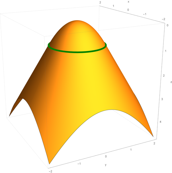
The code that I used to produce the above picture is as follows.
plotSampleggc =
 Show[plotSamplegg,
  ParametricPlot3D[{Cos[t], Sin[t], 1}, {t, 0, 2 Pi},
   PlotStyle -> {RGBColor[0, 0.5, 0], Thickness[0.01]},
   PlotPoints -> 200],
  AxesLabel -> {"x", "y", "z"}, BoxRatios -> {1, 1, 1},
  ImageSize -> 600,
  ViewPoint -> {-2.8517, -1.4654, -1.0818},
  ViewVertical -> {0.2844, 0.1461, -0.9475}]
You can copy and paste this code directly into your Mathematica notebook.
-
In this item I will present how to export pictures from Mathematica to display them on a website, or to use them in LaTeX files.
-
When exporting graphics, the first thing to be aware of is where on your computer the graphics will be exported. Mathematica provides several commands for checking that.
First, it is always good to know where is your Mathematica notebook located on your computer. That is done by executing
NotebookDirectory[]
Sometimes it even good to know what is the name of your Mathematica notebook
NotebookFileName[]
You can ask Mathematica where, by default, it exports files by executing
Directory[]
To tell Mathematica to exports files in the same directory where your current Mathematica notebook resides execute
SetDirectory[NotebookDirectory[]]
Instead of NotebookDirectory[] you can put any specific directory, like
SetDirectory["C:\\Dropbox"]
-
With two dimensional graphics exporting graphics is easy. When you create the graphics in Mathematica name it, for example myplot. Then, to export this graphics as a PNG file use
Export["myplot.png", myplot]
You can use different options in Export[]. I often like to control the size and the resolution of the exported picture:
Export["myplot.png", myplot,
ImageSize -> 600, ImageResolution -> 600]
Instead of PNG, one can use JPEG, GIF, EPS, SVG, PDF.
-
When exporting three-dimensional graphics, the simple form of the Export[] command may not preserve the exact orientation and appearance of the graphics as displayed in Mathematica. Below is a reliable workaround to address this issue.
-
First, create and name the graphics as shown in the example below:
Clear[ff]; ff[x_, y_] := Piecewise[{{x^2 + y^2, x^2 + y^2 <= 1}, {Sqrt[x^2 + y^2], x^2 + y^2 > 1}}]; plotSampleff = Plot3D[ff[x, y], {x, -2, 2}, {y, -2, 2}, PlotRange -> All, AxesLabel -> {"x", "y", "z"}, PlotPoints -> 200, Mesh -> None, Exclusions -> None, BoxRatios -> {1, 1, 1}, ImageSize -> 600, ViewPoint -> {-2.85169, -1.46541, -1.08185}, ViewVertical -> {0.284368, 0.14613, -0.947513}] -
Next, extract the Options from the created graphics. To do this:
- Copy the graphics that you created (using the name is not enough, copy the created picture) and paste it into a new command line.
- Append //Options to the copied image.
-
Assign the resulting options a name (I like using opts) for later use, like in the picture below:
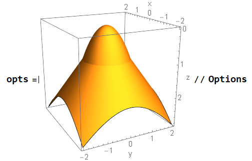
-
Finally, use the Export[] command with Show[] to ensure all options are preserved:
Export["plotSampleff.png", Show[plotSampleff, opts],
  ImageSize -> 600, ImageResolution -> 600]
This approach ensures that the exported graphics retain the same orientation, viewpoint, and appearance as in the Mathematica notebook.
-
- We continued with Example 3 in The Method of Characteristics: Burgers' equation. Read its own webpage Burgers' equation.
- I have posted three problems for Assignment 1 in Discussions on Canvas. All three problems involve the Method of Characteristics. Problem 3 focuses on Burgers' equation, for which a thorough review of the webpage Burgers' equation is essential. Additionally, The Method of Characteristics is a required reading for all three problems.
- Please post your comments, questions, and suggested corrections for the website content in Discussions on Canvas. For specific questions on your work for the assignment, stop by my office hours.
- At the end of the day today I posted Assignment 1 in Assignments on Canvas.
- We continued with Example 3 in The Method of Characteristics: Burgers' equation. Read its own webpage Burgers' equation.
- Today we did Problem 6 in The Method of Characteristics.
- We started work on Example 3 in The Method of Characteristics: Burgers' equation. Which has its own webpage.
-
Today we did Problem 8 in
The Method of Characteristics. This is the Problem:
-
Solve the following first order PDE
\begin{equation*}
x^2 u_x(x,y) + u_y(x,y) = 0 \quad \text{in} \quad U \subseteq \bigl\{(x,y) \in \mathbb R^2 : y \gt 0 \bigr\}
\end{equation*}
subject to the boundary condition
\begin{equation*}
u(x,0) = f(x) \quad \text{for} \quad x \in \mathbb R.
\end{equation*}
Notice that the domain $U$ is not given in the problem.
- For an arbitrary differentiable function $f$ find the solution $u(x,y)$ of the above problem and determine its maximum domain $U\subseteq \bigl\{(x,y) \in \mathbb R^2 : y \gt 0 \bigr\}$.
- Under which condition on $f$ the solution $u(x,y)$ will be defined on $\bigl\{(x,y) \in \mathbb R^2 : y \gt 0 \bigr\}$.
-
Solution. We solved characteristic equations
\[
X'(s) = \bigl(X(s)\bigr)^2, \quad Y'(s) = 1, \quad \text{and} \quad Z'(s) = 0,
\]
subject to initial conditions
\[
X(0) = \xi, \quad Y(0) = 0, \quad \text{and} \quad Z(0) = f(\xi).
\]
We found that the solution is
\[
X(s) = \frac{\xi }{1-\xi s}, \quad Y(s) = s, \quad \text{and} \quad Z(s) = f(\xi).
\]
In fact, the solution depends on \(\xi\) as well. So, the solution, properly written is
\[
X(s,\xi) = \frac{\xi }{1-\xi s}, \quad Y(s,\xi) = s, \quad \text{and} \quad Z(s,\xi) = f(\xi).
\]
These formulas hide the solution \(u(x,y)\).
Recall how we obtained the function \(Z(s)\), now \(Z(s,\xi)\): \[ Z(s,\xi) = u\bigl(X(s,\xi),Y(s,\xi)\bigr). \] In our case \[ u\left(\tfrac{\xi }{1-\xi s},s\right) = f(\xi). \] But we need the solution in terms of the coordinates \(x\) and \(y\). So, given a point \((x,y)\), we ask ourselves to calculate \(s\) and \(\xi\) that correspond to that point. We solve \[ x = \frac{\xi }{1-\xi s}, \quad y = s, \] for \(s\) and \(\xi\). The solution is \[ s = y, \quad \xi = \frac{x}{x y+1}. \] Hence, at the point \((x,y)\), the value of the solution \[ u(x,y) = f\left(\frac{x}{x y+1} \right). \]
- Verify. The initial condition \[ u(x,0) = f\left(\frac{x}{x 0+1} \right) = f(x). \] Partial derivatives: \begin{align*} u_x(x,y) & = f^\prime\left(\frac{x}{x y+1} \right) \frac{1}{(x y+1)^2}, \\ u_y(x,y) & =- f^\prime\left(\frac{x}{x y+1} \right) \frac{x^2}{(x y+1)^2}. \end{align*} And finally PDE: \[ x^2 u_x(x,y) + u_y(x,y) = x^2 f^\prime\left(\frac{x}{x y+1} \right) \frac{1}{(x y+1)^2} - f^\prime\left(\frac{x}{x y+1} \right) \frac{x^2}{(x y+1)^2} = 0. \]
-
Solve the following first order PDE
\begin{equation*}
x^2 u_x(x,y) + u_y(x,y) = 0 \quad \text{in} \quad U \subseteq \bigl\{(x,y) \in \mathbb R^2 : y \gt 0 \bigr\}
\end{equation*}
subject to the boundary condition
\begin{equation*}
u(x,0) = f(x) \quad \text{for} \quad x \in \mathbb R.
\end{equation*}
Notice that the domain $U$ is not given in the problem.
- I updated the post from Monday, January 13, 2025.
- Today we presented a general strategy for solving quasilinear partial differential equation: \begin{equation*} A\bigl(x,y,u(x,y)\bigr) \, u_x(x,y) + B\bigl(x,y,u(x,y)\bigr) \, u_y(x,y) = C\bigl(x,y,u(x,y)\bigr) \end{equation*} subject to the initial condition \begin{equation*} u(x,0) = f(x), \quad x \in \mathbb R, \end{equation*} where \(A, B, C\) are given real functions of three variables \(x,y,z\), \(f\) is a given real function of one variable \(x\) and \(u\) is an unknown function of two variables \(x,y\). The objective is to find a formula for \(u\) in terms of \(A, B, C\) and \(f\). For simplicity we assume that the given functions \(A\), \(B\) and \(C\) are smooth functions defined on \({\mathbb{R}}^3\) with the values in \(\mathbb R\) and that the given function \(f\) is a smooth function defined on \(\mathbb R\) with the values in \(\mathbb{R}\). Read more at my webpage The Method of Characteristics.
-
Today we solved the following first order PDE
\begin{equation*}
\frac{\partial u}{\partial x}(x,y) - \frac{\partial u}{\partial y}(x,y) = 0
\quad \text{where} \quad (x,y) \in \mathbb R^2
\end{equation*}
subject to the boundary condition
\begin{equation*}
u(x,0) = f(x), \quad \text{for} \quad x \in \mathbb R.
\end{equation*}
- Since the Partial Differential Equation is homogeneous, that is the expression with the first order derivatives equals \(0\), it is reasonable to expect that along some curves in the \(xy\)-plane there is no change in values of \(u(x,y)\). Let us look for those curves.
- Let \[ x = X(s), \qquad y = Y(s), \] be parametric equations of a curve in \(xy\)-plane. Now we focus on the values of \(u(x,y)\) along this curve. We consider the following function of \(s\): \[ u\bigl(X(s), Y(s) \bigr). \]
- Using the chain rule for multivariable functions, the derivative of this function of \(s\) is \[ \frac{d}{ds} u\bigl(X(s), Y(s) \bigr) = \frac{\partial u}{\partial x}\bigl(X(s), Y(s) \bigr) X'(s) + \frac{\partial u}{\partial y}\bigl(X(s), Y(s) \bigr) Y'(s). \] Compare the last expression to the given Partial Differential Equation. Recall that we are just experimenting with the functions \(X(s)\) and \(Y(s)\); we can choose these functions to be any differentiable functions. By setting \[ X'(s) = 1 \qquad \text{and} \qquad Y'(s) = -1, \] we get \begin{align*} \frac{d}{ds} u\bigl(X(s), Y(s) \bigr) & = \frac{\partial u}{\partial x}\bigl(X(s), Y(s) \bigr) X'(s) + \frac{\partial u}{\partial y}\bigl(X(s), Y(s) \bigr) Y'(s) \\ & = \frac{\partial u}{\partial x}\bigl(X(s), Y(s) \bigr) - \frac{\partial u}{\partial y}\bigl(X(s), Y(s) \bigr) = 0. \end{align*}
- Thus, there is no change along the curve determined by the parametric equations \(x = X(s)\), \(y = Y(s) \). To get useful solutions for \(X(s)\) and \(Y(s)\) we choose the initial conditions: \(X(0) = \xi\) and \(Y(0) = 0\). The reason for this choice is that from the initial values for the unknown \(u(x,y)\) we know the values \(u(\xi,0) = f(\xi)\). (A comment about my choice of notation: Instead of \(x\), I use \(\xi\) because \(x\) is often used as a general variable. The Greek lowercase letter \(\xi\) serves as a Greek counterpart to \(x\).) The nature of \(\xi\) here is that it is arbitrary real number, but fixed for now.
- The solution of the initial value problem \[ X'(s) = 1, \quad X(0) = \xi, \] is \[ X(s) = s + \xi. \] The solution of the initial value problem \[ Y'(s) = -1, \quad Y(0) = 0, \] is \[ Y(s) = - s. \]
- Thus, along the line \(x=s+\xi, \ y= -s\), where \(s\in\mathbb{R}\) and \(\xi\) is fixed, the function \(u(x,y)\) is constant. In other words, with fixed \(\xi\), if \(x+y = \xi\), we have that \(u(x,y)\) is constant. Therefore, if \(x+y = \xi\), we have \[ u(x,y) = u(\xi,0) = f(\xi) = f(x+y). \] Thus, the solution to the given Partial Differential Equation with the given Initial Values is \[ u(x,y) = f(x+y). \]
-
Recall the post of Saturday, January 11, 2025. We introduced the unknown function \(u(x,t)\) as follows \[ u(x,t) = \biggl({\huge e}^{^{\Large t \mkern 0.5mu \frac{d}{dx}}}\biggr) f(x), \quad \normalsize \text{where} \quad \large x, t \in \mathbb{R}. \] For this function we established that it satisfies the initial value problem for the following partial differential equation: \[ \frac{\partial u}{\partial t}(x,t) = \frac{\partial u}{\partial x}(x,t), \qquad u(x,0) = f(x). \] Here, instead of the variable \(y\), we use the variable \(t\). The reason for this is that in the content of Saturday's post this variable stands for time. Sometimes the equations studied in Saturday's post are called evolution equations; meaning evolution in time.
However, the names of variables are interchangeable. Therefore, the equation that we solved today gives us the solution of the equation that we established on Saturday.
The solution obtained today gives us the function \(u(x,t)\) that we introduced on Saturday: \[ u(x,t) = f(x+t). \]
Combining the last formula with the meaning of \(u(x,t)\) from Saturday: \[ u(x,t) = \biggl({\huge e}^{^{\Large t \mkern 0.5mu \frac{d}{dx}}}\biggr) f(x), \quad \normalsize \text{where} \quad \large x, t \in \mathbb{R}. \] we have the formula for the exponential function with \(t \frac{d}{dx}\) in the exponent: \[ \biggl({\huge e}^{^{\Large t \mkern 0.5mu \frac{d}{dx}}}\biggr) f(x) = f(x+t), \quad \text{where} \quad \large x, t \in \mathbb{R}. \] Thus, for each \(t\in\mathbb{R}\) the transformation \(\displaystyle {\huge e}^{^{\Large t \mkern 0.5mu \frac{d}{dx}}}\) acts on a function \(f(x)\) by shifting it's graph horizontally. The shift is to the left if \(t \gt 0\) and the shift is to the right if \(t \lt 0\).
- Now that we have established the formula \[ \biggl({\huge e}^{^{\Large t \mkern 0.5mu \frac{d}{dx}}}\biggr) f(x) = f(x+t), \quad \text{where} \quad x, t \in \mathbb{R}, \] we can draw a fascinating analogy with the standard exponential function from calculus. For real numbers \(a, c \in \mathbb{R}\), the standard exponential function satisfies: \[ {\Large c} \mkern 2mu {\huge e}^{^{\Large a \mkern 0.75mu t}} = \Bigl( {\huge e}^{^{\Large t \mkern 0.75mu a}} \Bigr) {\Large c}. \] Here, the expression \(\displaystyle \bigl( {\Large e}^{^{\Large t \mkern 0.75mu a}} \bigr) c\) is analogous to \[ \biggl({\huge e}^{^{\Large t \mkern 0.5mu \frac{d}{dx}}}\biggr) f(x), \] where \(\frac{d}{dx}\) plays the role of \(a\), and \(f(x)\) corresponds to \(c\).
- This analogy extends to the derivatives at \(t=0\). Consider the derivative of \(\displaystyle \bigl( {\Large e}^{^{\Large t \mkern 0.75mu a}} \bigr) {\large c}\) at \(t = 0\): \[ \lim_{t\to 0} \frac{\bigl(e^{t \mkern 0.75mu a} \bigr) c - c}{t} = c \lim_{t\to 0} \frac{e^{a \mkern 0.75mu t} - 1}{t} = c \mkern 2mu a = a \mkern 2mu c. \] The analogous computation for \(\displaystyle \Bigl({\Large e}^{^{\Large t \mkern 0.5mu \frac{d}{dx}}}\Bigr) f(x)\) gives: \[ \lim_{t\to 0} \frac{\Bigl({\Large e}^{^{\Large t \mkern 0.5mu \frac{d}{dx}}}\Bigr) f(x) - f(x)}{t} = \lim_{t\to 0} \frac{f(x+t) - f(x)}{t} = \frac{d}{dx} f(x). \] Notice the structure of the final terms in the last two displayed formulas: \(\frac{d}{dx}\) plays the role of \(a\), and \(f(x)\) corresponds to \(c\). This shows how the operator exponential \({\huge e}^{^{\Large t \mkern 0.5mu \frac{d}{dx}}}\) parallels the familiar exponential function in calculus.
- The analogy presented here has inspired a significant amount of research in mathematical analysis. This subfield is known as the theory of operator semigroups.
- The story that I am telling in this post fascinated me when I saw it for the first time as an undergraduate student a half-century ago.
-
In this item we review the most fundamental Initial Value Problem for Ordinary Differential Equations. Let \(a \in \mathbb{R}\) be an arbitrary real number.
- In calculus we studied the following problem: Find a function \(y(t)\) that satisfies the initial value problem \[ \Large \frac{dy}{dt}(t) = a \mkern 2mu y(t), \qquad y(0) = 1. \] A key topic in calculus is that this problem has a unique solution, given by the exponential function \[ \Large y(t) = e^{a \mkern 1.5mu t}, \quad \normalsize \text{where} \quad \Large t \in \mathbb{R}. \]
- More generally, one can consider the initial value problem for any \(c \in \mathbb{R}\): Find \(y(t)\) that solves \[ \Large \frac{dy}{dt}(t) = a \mkern 2mu y(t), \qquad y(0) = c. \] Again, in calculus we established that the unique solution to this problem is \[ \Large y(t) = c \mkern 2mu e^{a \mkern 1.5mu t}, \quad \normalsize \text{where} \quad \Large t \in \mathbb{R}. \]
- The problems stated in the preceding items are the simplest initial value problems for ordinary differential equations. Their importance lies in the fact that these problems describe the exponential growth or decay, a phenomenon commonly observed in nature.
- Given the importance and fundamental nature of the Initial Value Problems presented in the preceding item, courses on Ordinary Differential Equations or the second quarter course of Linear Algebra often explore a generalized version of these Initial Value Problems for square matrices. This exploration typically occurs during an in-depth study of matrix diagonalization. I do this in my Math 304, see the end of the post on Wednesday, October 9, 2024, starting with Problem 5 on Assignment 1 and the posts on Thursday, October 10, 2024, and Friday, October 11, 2024.
-
In this item we state the Matrix Version of the Initial Value Problem presented in the above item. Let \(n \in \mathbb{N}\) be a positive integer and \(A \in \mathbb{R}^{n\times n}\) is a square matrix.
- Find an \(n\times n\) matrix valued function \(Y(t)\) that satisfies the initial value problem \[ \Large \frac{dY}{dt}(t) = A \mkern 2mu Y(t), \qquad Y(0) = I_n. \] Here, \(I_n\) is the \(n\times n\) identity matrix. By definition, the solution of this Matrix Initial Value Problem is the Matrix Exponential Function \[ \Large Y(t) = {\huge e}^{^{{\Large A} \mkern 1.5mu t}}, \quad \normalsize \text{where} \quad \normalsize t \in \mathbb{R}. \]
-
For example, you can verify that
\[
{\Huge e}^{^{
\begin{bmatrix} 0 & -1 \\ 1 & 0 \end{bmatrix}
{\Large t}}} = \begin{bmatrix}
\cos(t) & -\sin(t) \\[5pt]\sin(t) & \cos(t)
\end{bmatrix},
\]
\[
{\Huge e}^{^{\begin{bmatrix} -1 & 2 \\ 0 & 1 \end{bmatrix}{\Large t}}} = \left[\!\begin{array}{cc}
e^{-t} &
e^{t} - e^{-t} \\[5pt] 0 &
e^{t}
\end{array}\!\right],
\]
\[
{\Huge e}^{^{\left[\begin{array}{ccc}
0 & 1 & 0 \\
0 & 0 & 2 \\
0 & 0 & 0 \\
\end{array}\right] {\Large t}}} =
\left[\!\begin{array}{ccc}
1 & t & t^2 \\
0 & 1 & 2t \\
0 & 0 & 1 \\
\end{array}\!\right].
\]
I say "you can verify that". I need to disclose that this is quite a bit of work. For example, to verify \[ {\Huge e}^{^{ \begin{bmatrix} 0 & -1 \\ 1 & 0 \end{bmatrix} {\Large t}}} = \begin{bmatrix} \cos(t) & -\sin(t) \\[5pt]\sin(t) & \cos(t) \end{bmatrix}, \] we need to verify that \[ \begin{bmatrix} \cos(0) & -\sin(0) \\[5pt]\sin(0) & \cos(0) \end{bmatrix} = \begin{bmatrix} 1 & 0 \\[5pt] 0 & 1 \end{bmatrix}. \] Ok, this is straightforward from the definitions of trigonometric functions. And we need to verify \[ \frac{d}{dt} \begin{bmatrix} \cos(t) & -\sin(t) \\[5pt]\sin(t) & \cos(t) \end{bmatrix} = \begin{bmatrix} 0 & -1 \\ 1 & 0 \end{bmatrix} \begin{bmatrix} \cos(t) & -\sin(t) \\[5pt]\sin(t) & \cos(t) \end{bmatrix}, \] which is an exercise in trigonometric derivatives and matrix multiplication.
- Instead of matrix valued functions, we can consider vector valued functions and formulate the Vector Initial Value Problem. Let \(\vec{\mathbf{v}}\) be a vector in \(\mathbb{R}^n\). Find a vector valued function \(\mathbf{y}(t)\) that solves the following vector initial value problem: \[ \Large \frac{d\vec{\mathbf{y}}}{dt}(t) = A \mkern 2mu \vec{\mathbf{y}}(t), \qquad \vec{\mathbf{y}}(0) = \vec{\mathbf{v}}. \] The unique solution of this initial value problem is \[ \Large \vec{\mathbf{y}}(t) = {\huge e}^{^{t \mkern 1mu {\Large A} }} \vec{\mathbf{v}}, \quad \normalsize \text{where} \quad \Large t \in \mathbb{R}. \]
-
Inspired by what is presented in Matrix Initial Value Problem we can answer the question: What is the exponential function of the derivative \(\frac{d}{dx}\)? That is we will give a meaning to
\[
{\Huge e}^{^{\Large t \mkern 0.5mu \frac{d}{dx}}}, \quad \normalsize \text{where} \quad \Large t \in \mathbb{R}.
\]
We proceed by analogy.
- Instead of an \(n\times n\) matrix \(A\) in Matrix Initial Value Problem we have the derivative \(\frac{d}{dx}\). The matrix \(A\) acts on vectors \(\vec{\mathbf{v}}\) in the vector space \(\mathbb{R}^n\). The derivative \(\frac{d}{dx}\) acts on the space of differentiable functions, for example on \(f(x)\).
- In Matrix Initial Value Problem we established that, for \(t\in \mathbb{R}\), \[ {\huge e}^{^{ {\Large t \mkern 1mu A} }} \] is an \(n\times n\) matrix. Then, in Vector Initial Value Problem, for a given vector \(\vec{\mathbf{v}} \in \mathbb{R}^n\), we established that \[ \Large \vec{\mathbf{y}}(t) = {\huge e}^{^{t \mkern 1mu {\Large A} }} \vec{\mathbf{v}} \] is the solution of the initial value problem \[ \large \frac{d\vec{\mathbf{y}}}{dt}(t) = A \mkern 2mu \vec{\mathbf{y}}(t), \qquad \vec{\mathbf{y}}(0) = \vec{\mathbf{v}}. \]
- To understand \[ {\Huge e}^{^{\Large t \mkern 0.5mu \frac{d}{dx}}}, \quad \normalsize \text{where} \quad \Large t \in \mathbb{R}, \] instead of a vector \(\vec{\mathbf{v}} \in \mathbb{R}^n\) we need to consider a differentiable function \(f(x)\) defined on \(\mathbb{R}\), that is defined and differentiable for all real numbers. Thus, instead of \[ \Large \vec{\mathbf{y}}(t) = {\huge e}^{^{t \mkern 1mu {\Large A} }} \vec{\mathbf{v}} \] we need to study the following function of \(x, t \in \mathbb{R}\): \[ u(x,t) =\mkern-16mu \underbrace{\biggl({\huge e}^{^{\Large t \mkern 0.5mu \frac{d}{dx}}}\biggr) f(x)}_{ \begin{array}{l} \text{this is a function of x and t;} \\ \text{we call it u(x,t)} \end{array}} \]
- Now, in the initial value problem \[ \large \frac{d\vec{\mathbf{y}}}{dt}(t) = A \mkern 2mu \vec{\mathbf{y}}(t), \qquad \vec{\mathbf{y}}(0) = \vec{\mathbf{v}}, \] instead of \(\vec{\mathbf{y}}(t)\) we have \(u(x,t)\), instead of \(A\) we have \(\frac{d}{dx}\), and instead if \(\vec{\mathbf{v}}\) we have \(f(x)\). Thus, to understand the expression \[ u(x,t) = \biggl({\huge e}^{^{\Large t \mkern 0.5mu \frac{d}{dx}}}\biggr) f(x), \] we need to solve the Initial Value Problem for the Partial Differential Equation \[ \Large \frac{\partial u}{\partial t}(x,t) = \frac{\partial u}{\partial x}(x,t), \qquad u(x,0) = f(x). \]
- Computer algebra system Mathematica will be very useful for the assignments in this class. To get started with Mathematica see my Mathematica page. A convenient way to get started is to watch the videos which are linked on my Mathematica page. Watching the movies is very helpful to get started with Mathematica efficiently! Mathematica is available in the computer labs in BH 215, HH 233 and BH 209/211A.
- During the first class I provide an overview of the course. As a guide to an overview I like to offer my explanations of the meaning of the words in the course title from the catalog. Today I offered the following explanation of the word equation: An equation is a mathematical expression which involves the equality sign and in which one component is considered unknown and the remaining components are considered known. To solve an equation means to find a formula for the unknown component in terms of the known quantities.
- Notice that in the explanation in the preceding item I use the concept of mathematical expression without explaining its meaning. As the Wikipedia page shows, an explanation of the concept mathematical expression is not simple.
- Today I offered the following definition of a Partial Differential Equation: A partial differential equation is an equation in which the unknown quantity is a function of several variables, and the equation involves this function, its partial derivatives, and other terms, called coefficients, which are specific or considered known. The coefficients can be constants or functions in the same independent variables as the unknown function.
- On Thursday, we will discuss special partial differential equations of the first order which can be solved using The Method of Characteristics. Reading the webpage The Method of Characteristics you will encounter several Partial Differential Equations. This pages also contains many ordinary differential equations; in fact systems of ordinary differential equations.
- My presentation of the Method of Characteristics differs from the presentation in the textbook. For comparison read Section 12.2.2 Method of Characteristics in the textbook. Suggested problems are 2, 3, 4, 5, 6, 7, 8 in Exercises 12.2, see Chapter 12 from the textbook.
- If you have any questions about the content or the organization of the class, please post them on Discussions on Canvas.
- The information sheet.
- We will start the class by studying the Method of characteristics for quasi-linear first order partial differential equations.
- My presentation of the Method of Characteristics differs from the presentation in the textbook. For comparison read Section 12.2.2 Method of Characteristics in the textbook. Suggested problems are 2, 3, 4, 5, 6, 7, 8 in Exercises 12.2, see Chapter 12 from the textbook.
- We will continue with the heat (or diffusion) equation. A derivation of the diffusion equation is here.
The animation below is obtained by solving that equation.
Place the cursor over the image to see the diffusion of the dye.

- Here is the complete list of all the webpages that I created for this class:
- Computer algebra system Mathematica will be very useful for the assignments in this class. You can start getting familiar with it. To get started with Mathematica see my Mathematica page. Please watch the videos that are on my Mathematica page. Watching the movies is very helpful to get started with Mathematica efficiently! Mathematica is available in the computer labs in BH 215, HH 233 and BH 209.
-
I recommend that you look into learning
LaTeX which is a superior typesetting system for writing mathematics. Not only that LaTeX is the best way to write mathematical content on computer, but it is the best way to display math on the Internet. All the mathematics that you see on my website is written in LaTeX. All the mathematics that you see on Wikipedia is written in LaTeX. In fact, if you go to a Wikipedia page with mathematics, on the line below the title, next to the Read button, you will find the Edit button. Clicking this Edit button will take you to the code for that webpage. You will see a lot of LaTeX code there. In fact, if you need exactly that formula, you can copy and paste it in your document.
- I created Getting Started with LaTeX page to help you with this.
- Here is a simple LaTeX sample document in which I prove an interesting inequality.
- If you need help starting with LaTeX, feel free to ask me for help. It is as important as learning one nice piece of mathematics. And I want to help you with that, not only because that is my job, but because I deeply believe that both math - through learning rigorous thinking - and professional writing skills - supported by rigorous thinking - will help you in your life more than anything else.
- I have noticed that many students use the online LaTeX editor Overleaf. I do not have any experience with Overleaf, except that I have seen that many students use it with nice results.
- LaTeX is just like a computer program that compiles into your mathematical document. As you probably know, ChatGPT is exceptionally good at writing code in all kinds of different languages. So, it is good at writing LaTeX code. If you are confused on how to do a particular task in LaTeX, you can ask ChatGPT for advise. All LaTeX related advise that I obtained from ChatGPT was superb. ChatGPT can also help you with Wolfram Mathematica code. Sometimes ChatGPT is sloppy, and makes mistakes, parenthesis not matching and stuff like that. If that happens, ask for corrections. It always helps to write very detailed user prompts.
-
Here is one example of my conversation with ChatGPT:

You:
Can you please write a complete LaTeX file with instructions on using basic mathematical operations, like fractions, sums, integrals, basic functions, like cosine, sine, and exponential function, and how to structure a document and similar features? Please explain the difference between the inline and displayed mathematical formulas. Please include examples of different ways of formatting displayed mathematical formulas. Please include what you think would be useful to a mathematics student. Also, can you please include your favorite somewhat complicated mathematical formula as an example of the power of LaTeX? I emphasize I want a complete file that I can copy into the LaTeX compiler and compile into a pdf file. Please ensure that your document contains the code for the formulas you are writing, which displays both as code separately from compiled formulas. Also, please double-check that your code compiles correctly. Remember that I am a beginner and cannot fix the errors. Please act as a concerned teacher would do.
This is the LaTeX document that ChatGPT produced base on the above prompt. Here is the compiled PDF document.
You can ask ChatGPT for specific LaTeX advise. To get a good response, think carefully about your prompt. Also, you can offer to ChatGPT a sample of short mathematical writing from the web or a book as a PNG file and it convert that writing to LaTeX. You can even try with neat handwriting. The results will of course depend on the clarity of the file, ChatGPT makes mistakes, but I found it incredibly useful.
- It is tempting to make LaTeX a mandatory tool for creating submissions in this class. However, I do not appreciate having mandates imposed on me; I prefer the freedom to think my own thoughts. An important part of a teacher's role is to encourage students to think their own thoughts, and imposing a mandate could undermine that principle.
- My one-page on the Power of Math.
- My one-page on Rigorous Reasoning.